ineqTrees provides tools for studying socioeconomic inequality in health outcomes with tree-based models. The package includes weighted rank and concentration-index utilities, inequality-aware split scoring, and wrappers for fitting greedy concentration-index trees and forests. Start with the inequality-aware party trees article for the main workflow, then see the tuning tutorial for cross-validating trees and forests and the plotting tutorial for customizing tree plots, node statistics, and labels.
Installation
You can install the development version of ineqTrees like so:
remotes::install_github("m-mburu/ineqTrees")Fitting a tree
The example below fits an inequality-aware greedy tree on a sample from the built-in kenya dataset. The response combines the ranking variable (wealth) and the health outcome (deadu5_num), while the split criterion is based on concentration-index reduction. The README uses shallow trees for readable figures; the main article shows examples with depth 3.
load data and set seed for reproducibility
if (requireNamespace("pkgload", quietly = TRUE) && file.exists("DESCRIPTION")) {
  suppressMessages(pkgload::load_all(export_all = FALSE))
} else {
  library(ineqTrees)
}
suppressPackageStartupMessages(library(data.table))
load("data/kenya.rda")
setDT(kenya)

set.seed(1)
Fit tree
This is a concentration-index tree, so the response is a two-column matrix of the ranking variable and the outcome. The rank_name and outcome_name arguments specify which columns of the data play those roles. The control argument uses greedy tree controls from ci_tree_control(), not conditional-inference test controls.
fit_tree <- ci_tree(
  formula = cbind(wealth, deadu5_num) ~ rural + ed + reg + unskilled,
  data = kenya,
  rank_name = "wealth",
  outcome_name = "deadu5_num",
  control = ci_tree_control(maxdepth = 2L)
)
#fit_tree
ci_tree_terminal_summary(fit_tree)
#>     node     n weight depth        ci outcome_mean outcome_percent
#>    <int> <int>  <num> <int>     <num>        <num>           <num>
#> 1:     3  2716   2716     2 0.2584802   0.02282769        2.282769
#> 2:     4  2050   2050     2 0.2667209   0.05707317        5.707317
#> 3:     6 12588  12588     2 0.2447775   0.07284716        7.284716
#> 4:     7  2689   2689     2 0.1695954   0.14168836       14.168836
#>                                                                                                                                                                                                                                                                                                                                                                  rule
#>                                                                                                                                                                                                                                                                                                                                                                <char>
#> 1:                                                                                                                          rural in {Urban} & reg in {Mombasa, Taita Taveta, Isiolo, Meru, Makueni, Nyeri, Kirinyaga, Kiambu, Trans Nzoia, Uasin Gishu, Nandi, Laikipia, Nakuru, Kajiado, Kericho, Bomet, Kakamega, Vihiga, Busia, Homa Bay, Migori, Kisii, Nairobi}
#> 2:                                                                                                          rural in {Urban} & reg in {Kwale, Kilifi, Tana River, Lamu, Garissa, Wajir, Mandera, Marsabit, Tharaka-Nithi, Embu, Kitui, Machakos, Nyandarua, Murang'a, Turkana, West Pokot, Samburu, Elgeyo-Marakwet, Baringo, Narok, Bungoma, Siaya, Kisumu, Nyamira}
#> 3: rural in {Rural} & reg in {Mombasa, Kwale, Kilifi, Lamu, Taita Taveta, Isiolo, Meru, Tharaka-Nithi, Embu, Kitui, Machakos, Makueni, Nyandarua, Nyeri, Kirinyaga, Murang'a, Kiambu, Trans Nzoia, Uasin Gishu, Elgeyo-Marakwet, Nandi, Baringo, Laikipia, Nakuru, Narok, Kajiado, Kericho, Bomet, Kakamega, Vihiga, Bungoma, Busia, Kisumu, Kisii, Nyamira, Nairobi}
#> 4:                                                                                                                                                                                                                                   rural in {Rural} & reg in {Tana River, Garissa, Wajir, Mandera, Marsabit, Turkana, West Pokot, Samburu, Siaya, Homa Bay, Migori}
readme_tree_plot(fit_tree, kenya, "deadu5_num")
Fitting a forest
The forest interface uses the same response specification, but averages predictions across many greedy concentration-index trees. The tuned workflow later in the README uses the same model family with cross-validation.
fit_forest <- ci_forest(
  formula = cbind(wealth, deadu5_num) ~ rural + ed + reg + unskilled,
  data = kenya,
  rank_name = "wealth",
  outcome_name = "deadu5_num",
  ntree = 10L,
  mtry = 1L,
  control = ci_tree_control(maxdepth = 2L)
)
fit_forest
Greedy concentration-index forest
Formula: cbind(wealth, deadu5_num) ~ rural + ed + reg + unskilled Criterion: CI Trees: 10
| ntree | mtry | type | n | mean_outcome | mean_prediction | outcome_ci | prediction_ci | mean_terminal_nodes | mean_max_depth |
|---|---|---|---|---|---|---|---|---|---|
| 10 | 1 | CI | 20043 | 0.074 | 0.074 | 0.311 | 0.075 | 3.6 | 2 |
Forest summary
ci_forest_summary(fit_forest)
#>    ntree  mtry   type     n mean_outcome mean_prediction outcome_ci
#>    <int> <int> <char> <int>        <num>           <num>      <num>
#> 1:    10     1     CI 20043   0.07369156      0.07368004  0.3114896
#>    prediction_ci mean_terminal_nodes mean_max_depth
#>            <num>               <num>          <num>
#> 1:    0.07545951                 3.6              2
Parallel execution patterns
ineqTrees uses the future ecosystem for optional parallel work and never sets the future plan inside model functions. Choose one layer at a time: direct forest fitting, custom tuning tasks, or tidymodels resamples.
old_plan <- future::plan()
future::plan(future::multisession, workers = 2)
on.exit(future::plan(old_plan), add = TRUE)

fit_forest <- ci_forest(
  formula = cbind(wealth, deadu5_num) ~ rural + ed + reg + unskilled,
  data = kenya,
  rank_name = "wealth",
  outcome_name = "deadu5_num",
  ntree = 50L,
  parallel = TRUE
)
old_plan <- future::plan()
future::plan(future::multisession, workers = 2)
on.exit(future::plan(old_plan), add = TRUE)

forest_tune_grid <- ci_tree_control_grid(
  minsplit = 100L,
  minbucket = c(50L, 100L),
  maxdepth = 1:2,
  mtry = c(1L, 2L),
  ntree = c(10L, 50L)
)

forest_tuning <- tune_ci_forest(
  formula = cbind(wealth, deadu5_num) ~ rural + ed + reg + unskilled,
  data = kenya,
  rank_name = "wealth",
  outcome_name = "deadu5_num",
  control_grid = forest_tune_grid,
  v = 5L,
  parallel_over = "tuning"
)
old_plan <- future::plan()
future::plan(future::multisession, workers = 2)
on.exit(future::plan(old_plan), add = TRUE)

forest_tuned <- tune::tune_grid(
  forest_wf,
  resamples = tree_folds,
  grid = forest_grid,
  metrics = yardstick::metric_set(ci_gain_tuning, yardstick::rmse),
  control = tune::control_grid(parallel_over = "resamples")
)
Fit a surrogate tree to forest predictions
The surrogate is a greedy concentration-index tree that approximates the predictions of the fitted forest. ci_forest_surrogate() adds the forest predictions to the analysis data and fits the surrogate with the same rank and predictor variables.
forest_surrogate <- ci_forest_surrogate(
  fit_forest,
  data = kenya,
  formula = cbind(wealth, deadu5_num) ~ rural + ed + reg + unskilled,
  rank_name = "wealth",
  prediction_name = "forest_risk",
  control = ci_tree_control(maxdepth = 2L)
)

surrogate_tree <- forest_surrogate$fit
surrogate_data <- forest_surrogate$data
#surrogate_tree
plot
readme_tree_plot(
  surrogate_tree,
  surrogate_data,
  outcome_name = "forest_risk",
  outcome_label = "Predicted risk"
)
SHAP-based decomposition
Approximate SHAP values with shapr::explain(), using a prediction wrapper that returns the predicted outcome for each observation, then decompose the concentration index of those predicted risks with shap_conc_decomp(). See the SHAP-based decomposition article for the full walkthrough across ci_tree(), ci_forest(), tidymodels-backed forests, and ordinary ranger models.
The model does not have to be an ineqTrees forest. shap_conc_decomp() only needs three things: SHAP values, the socioeconomic ranking variable, and the model’s predicted risk. That means the same step also works after fitting an ordinary prediction model, for example a ranger random forest tuned with tidymodels for risk of under-five death.
library(tidymodels)
library(ranger)

ranger_data <- as.data.frame(
  kenya[, c("wealth", "deadu5_num", readme_predictors), with = FALSE]
)
ranger_data$deadu5 <- factor(
  ifelse(ranger_data$deadu5_num == 1, "died", "alive"),
  levels = c("died", "alive")
)

ranger_risk_predict <- function(object, newdata) {
  prob <- predict(object, new_data = as.data.frame(newdata), type = "prob")
  as.numeric(prob$.pred_died)
}

ranger_folds <- vfold_cv(ranger_data, v = 5, strata = deadu5)

ranger_spec <- rand_forest(
  trees = 500,
  mtry = tune(),
  min_n = tune()
) %>%
  set_engine("ranger", probability = TRUE) %>%
  set_mode("classification")

ranger_wflow <- workflow() %>%
  add_model(ranger_spec) %>%
  add_formula(deadu5 ~ rural + ed + reg + unskilled)

ranger_grid <- grid_regular(
  mtry(range = c(1L, length(readme_predictors))),
  min_n(range = c(5L, 40L)),
  levels = 3
)

ranger_tuning <- tune_grid(
  ranger_wflow,
  resamples = ranger_folds,
  grid = ranger_grid,
  metrics = metric_set(roc_auc, accuracy)
)

best_ranger <- finalize_workflow(
  ranger_wflow,
  select_best(ranger_tuning, metric = "roc_auc")
) %>%
  fit(data = ranger_data)

ranger_X <- ranger_data[, readme_predictors, drop = FALSE]
ranger_eval_n <- min(400L, nrow(ranger_data))
ranger_rows <- sort(sample.int(nrow(ranger_data), ranger_eval_n))
ranger_X_eval <- ranger_X[ranger_rows, , drop = FALSE]
ranger_pred_eval <- ranger_risk_predict(best_ranger, ranger_X_eval)

ranger_shap <- estimate_shapr_values(
  object = best_ranger,
  x_train = ranger_X,
  x_explain = ranger_X_eval,
  pred_wrapper = ranger_risk_predict,
  seed = 20260328
)

ranger_decomp <- shap_conc_decomp(
  shap = ranger_shap,
  rank = ranger_data$wealth[ranger_rows],
  prediction = ranger_pred_eval
)
ranger_shap_diagnostics <- as.data.frame(ranger_decomp$diagnostics)
ranger_shap_contrib_table <- as.data.frame(ranger_decomp$contributions)
ranger_shap_contrib_table <- ranger_shap_contrib_table[
  order(-ranger_shap_contrib_table$abs_contribution),
  ,
  drop = FALSE
]
knitr::kable(
  ranger_shap_diagnostics,
  digits = 3,
  caption = "Ranger SHAP decomposition diagnostics"
)| n | weight_sum | type | mean_prediction | concentration_index | signed_concentration_index | score_direction | shap_sum | additivity_gap | centered_rank_sum | prediction_source |
|---|---|---|---|---|---|---|---|---|---|---|
| 400 | 400 | CI | 0.073 | 0.105 | -0.105 | -1 | 0.105 | 0 | 0 | prediction |
Ranger SHAP decomposition diagnostics
knitr::kable(
  ranger_shap_contrib_table,
  digits = 3,
  caption = "Ranger SHAP-based concentration-index contributions"
)| feature | D_k_SHAP | pct_contribution | abs_contribution |
|---|---|---|---|
| rural | 0.041 | 39.246 | 0.041 |
| ed | 0.027 | 25.152 | 0.027 |
| unskilled | 0.020 | 18.679 | 0.020 |
| reg | 0.018 | 16.923 | 0.018 |
Ranger SHAP-based concentration-index contributions
library(ggplot2)
ggplot(
  ranger_shap_contrib_table,
  aes(
    x = stats::reorder(feature, pct_contribution),
    y = pct_contribution,
    fill = pct_contribution > 0
  )
) +
  geom_col(width = 0.7) +
  coord_flip() +
  scale_fill_manual(
    values = c("#2166ac", "#b2182b"),
    guide = "none"
  ) +
  labs(
    x = NULL,
    y = "Percentage contribution",
    title = "Ranger SHAP-based concentration-index decomposition"
  ) +
  theme_minimal(base_size = 12) +
  theme(panel.grid.minor = element_blank())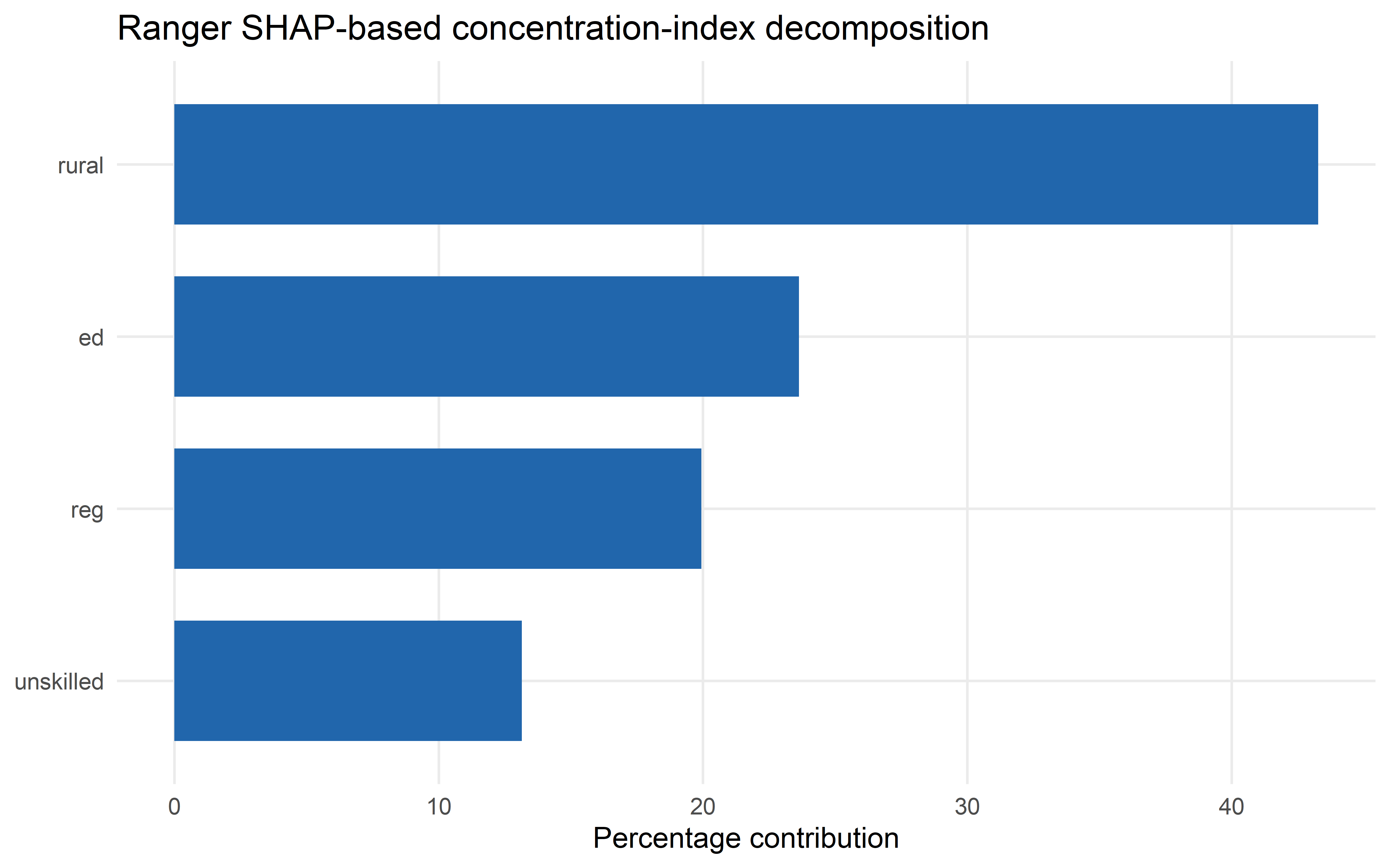
set.seed(20260328)
shap_eval_n <- min(400L, nrow(kenya))
shap_rows <- sort(sample.int(nrow(kenya), shap_eval_n))
forest_X <- kenya[, ..readme_predictors]
shap_X_eval <- forest_X[shap_rows, , drop = FALSE]
forest_pred_eval <- readme_forest_predict(fit_forest, shap_X_eval)
wealth_eval <- kenya$wealth[shap_rows]

forest_shap <- estimate_shapr_values(
  object = fit_forest,
  x_train = forest_X,
  x_explain = shap_X_eval,
  pred_wrapper = readme_forest_predict,
  seed = 20260328
)

decomp <- shap_conc_decomp(
  shap = forest_shap,
  rank = wealth_eval,
  prediction = forest_pred_eval
)

shap_diagnostics <- as.data.frame(decomp$diagnostics)
shap_contrib_table <- as.data.frame(decomp$contributions)
shap_contrib_table <- shap_contrib_table[
  order(-shap_contrib_table$abs_contribution),
  ,
  drop = FALSE
]
knitr::kable(
  shap_diagnostics,
  digits = 3,
  caption = "SHAP decomposition diagnostics"
)| n | weight_sum | type | mean_prediction | concentration_index | signed_concentration_index | score_direction | shap_sum | additivity_gap | centered_rank_sum | prediction_source |
|---|---|---|---|---|---|---|---|---|---|---|
| 400 | 400 | CI | 0.074 | 0.07 | -0.07 | -1 | 0.07 | 0 | 0 | prediction |
SHAP decomposition diagnostics
knitr::kable(
  shap_contrib_table,
  digits = 3,
  caption = "SHAP-based concentration-index contributions"
)| feature | D_k_SHAP | pct_contribution | abs_contribution |
|---|---|---|---|
| reg | 0.027 | 38.375 | 0.027 |
| rural | 0.017 | 24.640 | 0.017 |
| ed | 0.016 | 22.602 | 0.016 |
| unskilled | 0.010 | 14.383 | 0.010 |
SHAP-based concentration-index contributions
library(ggplot2)
ggplot(
  shap_contrib_table,
  aes(
    x = stats::reorder(feature, pct_contribution),
    y = pct_contribution,
    fill = pct_contribution > 0
  )
) +
  geom_col(width = 0.7) +
  coord_flip() +
  scale_fill_manual(
    values = c("#2166ac", "#b2182b"),
    guide = "none"
  ) +
  labs(
    x = NULL,
    y = "Percentage contribution",
    title = "SHAP-based concentration-index decomposition"
  ) +
  theme_minimal(base_size = 12) +
  theme(panel.grid.minor = element_blank())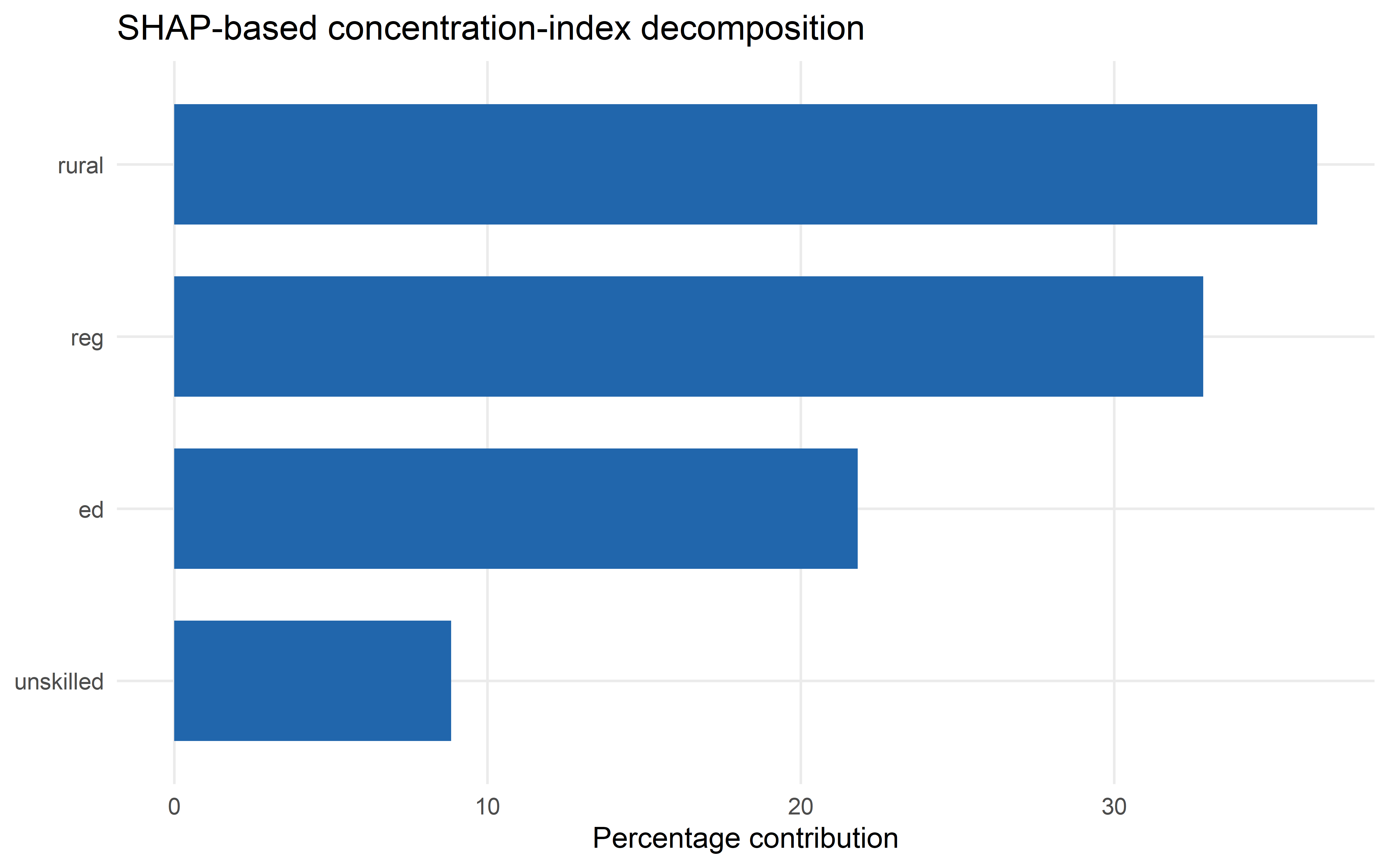
Tune tree hyperparameters
The package-native tuning workflow uses ci_tree_control_grid() to define candidate greedy controls and tune_ci_tree() to score them with cross-validation. Pass one or more concentration-index objectives through type, compute one or more metrics with metrics, and use control_ci_tune() when you want saved predictions, saved fits, or extraction hooks. The ci_collect_*() helpers read the result back in a stable shape.
tree_tune_grid <- ci_tree_control_grid(
  minsplit = 100L,
  minbucket = c(50L, 100L),
  maxdepth = c(1L, 2L),
  minprob = c(0.01, 0.05)
)
tree_tuning <- tune_ci_tree(
  formula = cbind(wealth, deadu5_num) ~ rural + ed + reg + unskilled,
  data = tuning_data,
  rank_name = "wealth",
  outcome_name = "deadu5_num",
  type = c("CI", "CIg"),
  control_grid = tree_tune_grid,
  v = 3L,
  strata = "deadu5_num",
  seed = 20260507,
  metrics = c("validation_gain", "relative_validation_gain", "brier"),
  refit = TRUE,
  control = control_ci_tune(save_pred = TRUE)
)
tree_tuning_best <- ci_select_best(
  tree_tuning,
  metric = "validation_gain"
)

tree_tuning_table <- readme_tuning_table(
  ci_fit_summary_table(
    tree_tuning,
    selected = tree_tuning_best,
    metrics = c(
      "train_gain",
      "validation_gain",
      "train_relative_gain",
      "relative_validation_gain"
    )
  ),
  columns = c(
    "type",
    "minsplit",
    "minbucket",
    "minprob",
    "maxdepth",
    "mean_root_objective",
    "mean_train_gain",
    "mean_validation_gain",
    "mean_validation_relative_gain"
  ),
  labels = c(
    "type",
    "minsplit",
    "minbucket",
    "minprob",
    "maxdepth",
    "mean_root_objective",
    "mean_train_gain",
    "mean_validation_gain",
    "mean_relative_validation_gain"
  )
)

knitr::kable(
  tree_tuning_table,
  digits = 3,
  caption = "Cross-validated greedy tree tuning results"
)| type | minsplit | minbucket | minprob | maxdepth | mean_root_objective | mean_train_gain | mean_validation_gain | mean_relative_validation_gain |
|---|---|---|---|---|---|---|---|---|
| CI | 100 | 50 | 0.01 | 1 | 0.398 | 0.208 | -0.017 | -0.104 |
| CIg | 100 | 100 | 0.01 | 2 | 0.031 | 0.009 | 0.001 | 0.035 |
Cross-validated greedy tree tuning results
tree_wide_metrics <- ci_collect_metrics(
  tree_tuning,
  metric = c("train_gain", "validation_gain"),
  format = "wide"
)

tree_saved_predictions <- ci_collect_predictions(tree_tuning)

knitr::kable(
  head(tree_wide_metrics[, .(
    grid_id,
    type,
    mean_train_gain,
    mean_validation_gain,
    std_err_validation_gain
  )]),
  digits = 3,
  caption = "Wide-format training and validation gain metrics collected from tree tuning"
)| grid_id | type | mean_train_gain | mean_validation_gain | std_err_validation_gain |
|---|---|---|---|---|
| 1 | CI | 0.208 | -0.017 | 0.027 |
| 2 | CI | 0.208 | -0.017 | 0.027 |
| 3 | CI | 0.208 | -0.017 | 0.027 |
| 4 | CI | 0.208 | -0.017 | 0.027 |
| 5 | CI | 0.247 | -0.023 | 0.035 |
| 6 | CI | 0.215 | -0.068 | 0.032 |
Wide-format training and validation gain metrics collected from tree tuning
readme_tree_plot(
  fit = tree_tuning$best_fit,
  data = tuning_data,
  outcome_name = "deadu5_num"
)
Tune forest hyperparameters
For forests, tune_ci_forest() uses the same greedy controls and adds ntree when that column is present in the tuning grid. Forest validation gain is computed by averaging held-out CI gain across each candidate forest’s internal tree partitions, while prediction metrics such as Brier score use the averaged forest predictions. Use parallel_over = "tuning" to parallelize grid/fold tasks, or parallel_over = "forest" to grow trees within each forest in parallel after setting a future plan.
forest_tune_grid <- ci_tree_control_grid(
  minsplit = 100L,
  minbucket = c(50L, 100L),
  maxdepth = c(1L, 2L),
  mtry = c(1L, 2L),
  ntree = c(10L, 20L),
  minprob = 0.01
)
forest_tuning <- tune_ci_forest(
  formula = cbind(wealth, deadu5_num) ~ rural + ed + reg + unskilled,
  data = tuning_data,
  rank_name = "wealth",
  outcome_name = "deadu5_num",
  type = c("CI", "CIg"),
  control_grid = forest_tune_grid,
  v = 3L,
  strata = "deadu5_num",
  seed = 20260508,
  metrics = c("validation_gain", "relative_validation_gain", "brier"),
  prediction_name = "forest_risk",
  parallel_over = "none",
  control = control_ci_tune(save_pred = TRUE),
  surrogate_control = ci_tree_control(maxdepth = 2L),
  refit = TRUE
)
forest_tuning_best <- ci_select_best(
  forest_tuning,
  metric = "validation_gain"
)

forest_tuning_table <- readme_tuning_table(
  ci_fit_summary_table(
    forest_tuning,
    selected = forest_tuning_best,
    metrics = c(
      "train_gain",
      "validation_gain",
      "train_relative_gain",
      "relative_validation_gain"
    )
  ),
  columns = c(
    "type",
    "ntree",
    "mtry",
    "minbucket",
    "maxdepth",
    "mean_root_objective",
    "mean_train_gain",
    "mean_validation_gain",
    "mean_percent_validation_gain"
  ),
  labels = c(
    "type",
    "ntree",
    "mtry",
    "minbucket",
    "maxdepth",
    "mean_root_objective",
    "mean_train_gain",
    "mean_validation_gain",
    "percent_validation_gain"
  )
)

knitr::kable(
  forest_tuning_table,
  digits = 3,
  caption = "Cross-validated greedy forest tuning results ranked by validation gain"
)| type | ntree | mtry | minbucket | maxdepth | mean_root_objective | mean_train_gain | mean_validation_gain | percent_validation_gain |
|---|---|---|---|---|---|---|---|---|
| CI | 20 | 2 | 50 | 1 | 0.397 | 0.008 | 0.012 | 3.055 |
| CIg | 20 | 1 | 50 | 2 | 0.031 | 0.003 | 0.001 | 4.456 |
Cross-validated greedy forest tuning results ranked by validation gain
forest_saved_predictions <- ci_collect_predictions(forest_tuning)
forest_brier <- ci_collect_metrics(
  forest_tuning,
  metric = "brier",
  format = "wide"
)

knitr::kable(
  head(forest_brier[, .(type, ntree, mtry, mean_brier, std_err_brier)]),
  digits = 3,
  caption = "Brier scores collected from the same forest tuning run"
)| type | ntree | mtry | mean_brier | std_err_brier |
|---|---|---|---|---|
| CI | 10 | 1 | 0.072 | 0.001 |
| CI | 10 | 1 | 0.073 | 0.001 |
| CI | 10 | 1 | 0.073 | 0.001 |
| CI | 10 | 1 | 0.073 | 0.001 |
| CI | 10 | 2 | 0.073 | 0.001 |
| CI | 10 | 2 | 0.073 | 0.001 |
Brier scores collected from the same forest tuning run
best_tuned_forest <- forest_tuning$best_fit
forest_surrogate_data <- forest_tuning$best_surrogate_data
forest_surrogate_fit <- forest_tuning$best_surrogate
readme_tree_plot(
  fit = forest_surrogate_fit,
  data = forest_surrogate_data,
  outcome_name = "forest_risk",
  outcome_label = "Predicted risk"
)