Inequality-aware party trees
Source:vignettes/inequality-aware-party-trees.Rmd
inequality-aware-party-trees.RmdIntroduction
ineqTrees is designed for a specific kind of applied
question: how is a health outcome distributed across a socioeconomic
ranking, and which subgroups account for the remaining inequality?
The package keeps three pieces of information together:
- a socioeconomic rank, such as household wealth;
- a health outcome, such as under-five death;
- predictors that define interpretable subgroups.
The examples below use the kenya dataset shipped with
the package. The data are simulated from a DHS-style child survival
setting, so they are useful for demonstrating the workflow without
requiring external survey files.
library(ineqTrees)
library(data.table)
#>
#> Attaching package: 'data.table'
#> The following object is masked from 'package:base':
#>
#>     %notin%

data(kenya, package = "ineqTrees")
setDT(kenya)
1. Prepare the analysis table
For a concentration-index tree, the response has two columns: the
socioeconomic ranking variable and the health outcome. Here,
wealth is the rank and deadu5_num is a binary
indicator for under-five death.
analysis_vars <- c(
  "wealth",
  "deadu5_num",
  "rural",
  "ed",
  "reg",
  "unskilled",
  "sample_weight"
)

kenya_child <- kenya[
  complete.cases(kenya[, ..analysis_vars]),
  ..analysis_vars
]

kenya_child[
  ,
  .(
    children = .N,
    mortality = mean(deadu5_num),
    mean_wealth = mean(wealth)
  ),
  by = rural
]
#>     rural children  mortality mean_wealth
#>    <fctr>    <int>      <num>       <num>
#> 1:  Rural    15277 0.08496433  -0.3046825
#> 2:  Urban     4766 0.03755770   0.5498055
For a fast vignette build we use a reproducible subset. In a real analysis you would normally fit the model to the full prepared survey table.
set.seed(20260512)
kenya_model <- kenya_child[
  sample.int(.N, min(1000L, .N))
]

predictors <- c("rural", "ed", "reg", "unskilled")
criterion_types <- c("CI", "CIg", "CIc", "L")
2. Measure socioeconomic inequality at the root
The concentration index summarizes whether the outcome is
concentrated among poorer or richer children after ordering observations
by the ranking variable. ci_root_impurity() computes the
unsplit/root objective with the same scoring convention used by tree and
forest tuning. Each criterion has its own root-node benchmark.
whole_sample_ci <- data.table(type = criterion_types)[
  ,
  .(
    root_ci_index = ci_root_impurity(
      data = kenya_model,
      rank_name = "wealth",
      outcome_name = "deadu5_num",
      weights = kenya_model$sample_weight,
      type = type
    )
  ),
  by = type
]
#> Warning: `type = "L"` uses observed socioeconomic levels rather than fractional
#> ranks. The first response column contains negative values; the
#> Erreygers-Kessels level-dependent index is intended for meaningful ratio-scale
#> socioeconomic levels such as income, consumption, or expenditure. Centered
#> wealth-index scores with negative values may be inappropriate for this
#> criterion. See https://doi.org/10.3390/ijerph14070673. This warning is shown
#> once per R session.

ci <- ci_factory("CI")

whole_sample_ci
#>      type root_ci_index
#>    <char>         <num>
#> 1:     CI    0.36764493
#> 2:    CIg    0.02496335
#> 3:    CIc    0.09985342
#> 4:      L    0.21587338
The root_ci_index is the baseline impurity before any
subgrouping. The same type argument appears in the tree and
tuning functions, so each fitted model should be compared with the root
benchmark for the same concentration-index criterion.
3. Fit trees with different concentration indices
ci_tree() can optimize several related
concentration-index objectives. This is important in applied work
because the preferred index depends on the outcome scale and on whether
the ranking variable should be treated as a fractional rank or as
observed socioeconomic levels.
-
"CI"is the standard concentration index. -
"CIg"is a generalized concentration index. -
"CIc"is a corrected concentration index for bounded outcomes. -
"L"uses the observed socioeconomic levels in the first response column.
You select the objective with the type argument. The
fitted objects have the same interface, so they can be printed,
summarized, validated, or plotted in the same way.
tree_control <- ci_tree_control(
  minsplit = 120,
  minbucket = 60,
  minprob = 0.05,
  maxdepth = 3
)

tree_by_type <- setNames(
  lapply(criterion_types, function(ci_type) {
    ci_tree(
      formula = cbind(wealth, deadu5_num) ~ rural + ed + reg + unskilled,
      data = kenya_model,
      rank_name = "wealth",
      outcome_name = "deadu5_num",
      weights = kenya_model$sample_weight,
      type = ci_type,
      control = tree_control
    )
  }),
  criterion_types
)

type_comparison <- rbindlist(lapply(names(tree_by_type), function(ci_type) {
  fit <- tree_by_type[[ci_type]]

  data.table(
    type = ci_type,
    terminal_nodes = length(partykit::nodeids(fit, terminal = TRUE)),
    validation_gain = ci_tree_validation_gain(
      fit = fit,
      new_data = kenya_model,
      rank_name = "wealth",
      outcome_name = "deadu5_num",
      weights = kenya_model$sample_weight,
      type = ci_type
    )
  )
}))

type_comparison[order(-validation_gain)]
#>      type terminal_nodes validation_gain
#>    <char>          <int>           <num>
#> 1:     CI              7      0.20872157
#> 2:      L              5      0.17779168
#> 3:    CIc              6      0.05039079
#> 4:    CIg              6      0.01259770
In this quick comparison, larger validation gain means the terminal-node partition removes more concentration-index impurity than the unsplit root in the same sample. In a final analysis, use cross-validation to select among indices and tree-size controls rather than choosing the largest in-sample score.
For the rest of the introduction we continue with the standard concentration index tree.
4. Fit a greedy concentration-index tree
ci_tree() grows a binary tree by looking for splits that
reduce within-node concentration-index impurity. The formula uses
cbind(wealth, deadu5_num) so the model knows both the
ranking variable and the outcome.
tree_fit <- ci_tree(
  formula = cbind(wealth, deadu5_num) ~ rural + ed + reg + unskilled,
  data = kenya_model,
  rank_name = "wealth",
  outcome_name = "deadu5_num",
  weights = kenya_model$sample_weight,
  type = "CI",
  control = tree_control
)

tree_fit
Greedy concentration-index tree
Formula:
cbind(wealth, deadu5_num) ~ rural + ed + reg + unskilled
Criterion: CI Tree size: 6 inner
nodes, 7 terminal nodes, max depth 3
| node | n | weight | depth | CI | outcome_mean | outcome_percent | rule |
|---|---|---|---|---|---|---|---|
| 8 | 77 | 66.17731 | 3 | 0.371 | 0.033 | 3.3 | reg in {Kwale, Lamu, Taita Taveta, Garissa, Isiolo, Meru, Kitui, Machakos, Nyandarua, Kirinyaga, Murang’a, Trans Nzoia, Baringo, Laikipia, Kajiado, Kakamega, Vihiga, Busia, Kisumu, Migori, Nairobi} & unskilled in {Yes} & reg in {Kitui, Machakos, Kakamega, Migori, Nairobi} |
| 12 | 249 | 234.02704 | 3 | 0.339 | 0.107 | 10.7 | reg in {Mombasa, Kilifi, Tana River, Wajir, Mandera, Marsabit, Tharaka-Nithi, Embu, Makueni, Nyeri, Kiambu, Turkana, West Pokot, Samburu, Uasin Gishu, Elgeyo-Marakwet, Nandi, Nakuru, Narok, Kericho, Bomet, Bungoma, Siaya, Homa Bay, Kisii, Nyamira} & unskilled in {No} & reg in {Tana River, Wajir, Mandera, Marsabit, Embu, Nyeri, Kiambu, Turkana, West Pokot, Samburu, Uasin Gishu, Elgeyo-Marakwet, Nandi, Nakuru, Narok, Siaya, Homa Bay, Nyamira} |
| 13 | 213 | 188.49032 | 2 | 0.195 | 0.173 | 17.3 | reg in {Mombasa, Kilifi, Tana River, Wajir, Mandera, Marsabit, Tharaka-Nithi, Embu, Makueni, Nyeri, Kiambu, Turkana, West Pokot, Samburu, Uasin Gishu, Elgeyo-Marakwet, Nandi, Nakuru, Narok, Kericho, Bomet, Bungoma, Siaya, Homa Bay, Kisii, Nyamira} & unskilled in {Yes} |
| 5 | 126 | 102.99408 | 3 | 0.011 | 0.008 | 0.8 | reg in {Kwale, Lamu, Taita Taveta, Garissa, Isiolo, Meru, Kitui, Machakos, Nyandarua, Kirinyaga, Murang’a, Trans Nzoia, Baringo, Laikipia, Kajiado, Kakamega, Vihiga, Busia, Kisumu, Migori, Nairobi} & unskilled in {No} & reg in {Kwale, Garissa, Meru, Vihiga, Busia, Kisumu, Migori, Nairobi} |
| 4 | 144 | 127.14356 | 3 | 0.000 | 0.000 | 0.0 | reg in {Kwale, Lamu, Taita Taveta, Garissa, Isiolo, Meru, Kitui, Machakos, Nyandarua, Kirinyaga, Murang’a, Trans Nzoia, Baringo, Laikipia, Kajiado, Kakamega, Vihiga, Busia, Kisumu, Migori, Nairobi} & unskilled in {No} & reg in {Lamu, Taita Taveta, Isiolo, Kitui, Machakos, Nyandarua, Kirinyaga, Murang’a, Trans Nzoia, Baringo, Laikipia, Kajiado, Kakamega} |
| 11 | 104 | 100.62121 | 3 | 0.000 | 0.000 | 0.0 | reg in {Mombasa, Kilifi, Tana River, Wajir, Mandera, Marsabit, Tharaka-Nithi, Embu, Makueni, Nyeri, Kiambu, Turkana, West Pokot, Samburu, Uasin Gishu, Elgeyo-Marakwet, Nandi, Nakuru, Narok, Kericho, Bomet, Bungoma, Siaya, Homa Bay, Kisii, Nyamira} & unskilled in {No} & reg in {Mombasa, Kilifi, Tharaka-Nithi, Makueni, Kericho, Bomet, Bungoma, Kisii} |
| 7 | 87 | 73.60556 | 3 | 0.000 | 0.000 | 0.0 | reg in {Kwale, Lamu, Taita Taveta, Garissa, Isiolo, Meru, Kitui, Machakos, Nyandarua, Kirinyaga, Murang’a, Trans Nzoia, Baringo, Laikipia, Kajiado, Kakamega, Vihiga, Busia, Kisumu, Migori, Nairobi} & unskilled in {Yes} & reg in {Kwale, Lamu, Taita Taveta, Garissa, Isiolo, Meru, Nyandarua, Kirinyaga, Murang’a, Trans Nzoia, Baringo, Laikipia, Kajiado, Vihiga, Busia, Kisumu} |
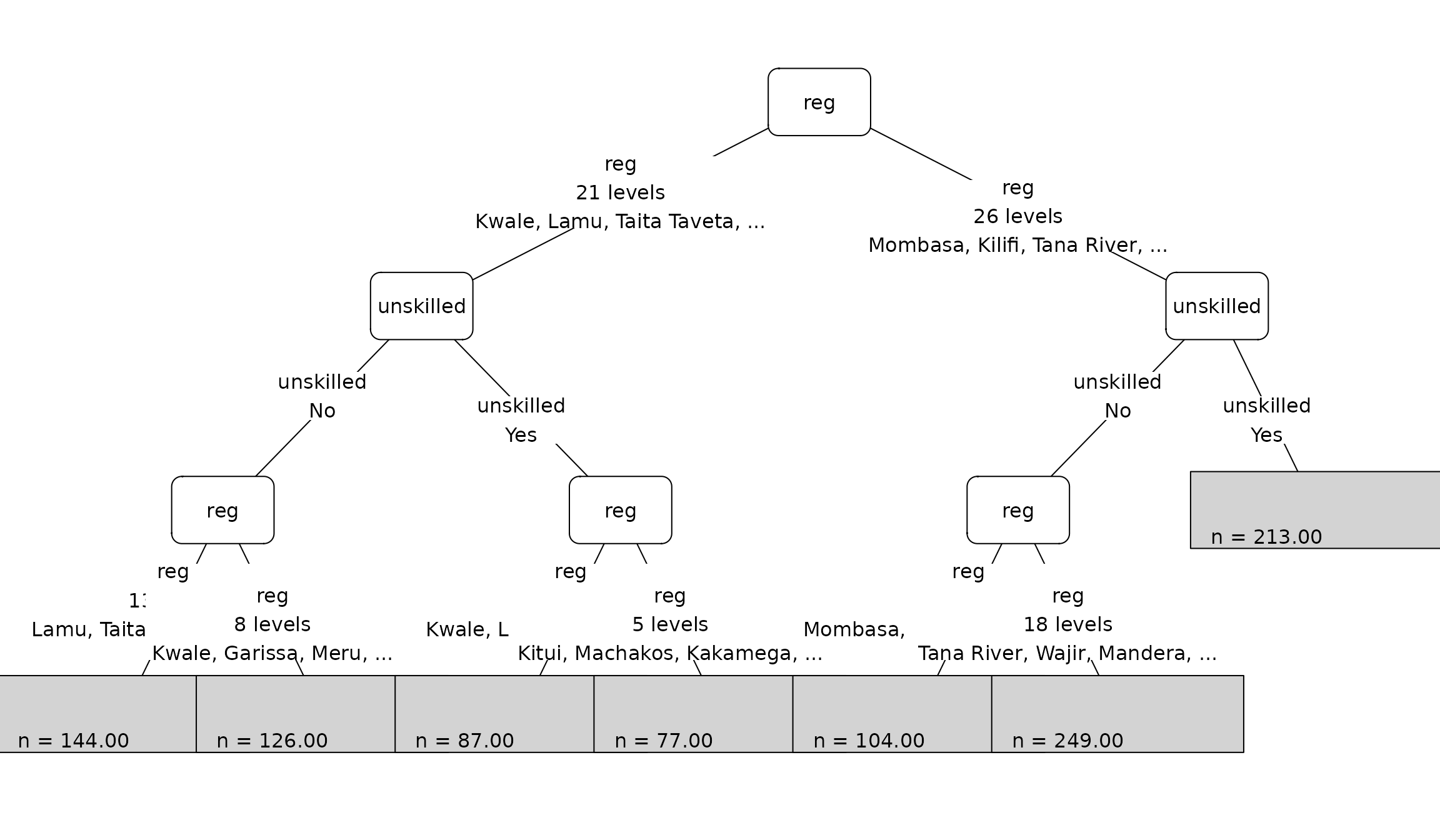
The printed tree shows the model objective, the number of terminal nodes, and a terminal-node summary. The most useful table for interpretation is often the terminal summary itself.
terminal_summary <- ci_tree_terminal_summary(tree_fit)

terminal_summary[
  order(-outcome_percent),
  .(node, n, depth, ci, outcome_percent, rule)
]
#>     node     n depth         ci outcome_percent
#>    <int> <int> <int>      <num>           <num>
#> 1:    13   213     2 0.19529952      17.2941102
#> 2:    12   249     3 0.33925108      10.6954095
#> 3:     8    77     3 0.37149505       3.2896765
#> 4:     5   126     3 0.01104352       0.8101999
#> 5:     4   144     3 0.00000000       0.0000000
#> 6:     7    87     3 0.00000000       0.0000000
#> 7:    11   104     3 0.00000000       0.0000000
#>                                                                                                                                                                                                                                                                                                                                                                                                                                                            rule
#>                                                                                                                                                                                                                                                                                                                                                                                                                                                          <char>
#> 1:                                                                                                                                                                                 reg in {Mombasa, Kilifi, Tana River, Wajir, Mandera, Marsabit, Tharaka-Nithi, Embu, Makueni, Nyeri, Kiambu, Turkana, West Pokot, Samburu, Uasin Gishu, Elgeyo-Marakwet, Nandi, Nakuru, Narok, Kericho, Bomet, Bungoma, Siaya, Homa Bay, Kisii, Nyamira} & unskilled in {Yes}
#> 2: reg in {Mombasa, Kilifi, Tana River, Wajir, Mandera, Marsabit, Tharaka-Nithi, Embu, Makueni, Nyeri, Kiambu, Turkana, West Pokot, Samburu, Uasin Gishu, Elgeyo-Marakwet, Nandi, Nakuru, Narok, Kericho, Bomet, Bungoma, Siaya, Homa Bay, Kisii, Nyamira} & unskilled in {No} & reg in {Tana River, Wajir, Mandera, Marsabit, Embu, Nyeri, Kiambu, Turkana, West Pokot, Samburu, Uasin Gishu, Elgeyo-Marakwet, Nandi, Nakuru, Narok, Siaya, Homa Bay, Nyamira}
#> 3:                                                                                                                                                                             reg in {Kwale, Lamu, Taita Taveta, Garissa, Isiolo, Meru, Kitui, Machakos, Nyandarua, Kirinyaga, Murang'a, Trans Nzoia, Baringo, Laikipia, Kajiado, Kakamega, Vihiga, Busia, Kisumu, Migori, Nairobi} & unskilled in {Yes} & reg in {Kitui, Machakos, Kakamega, Migori, Nairobi}
#> 4:                                                                                                                                                            reg in {Kwale, Lamu, Taita Taveta, Garissa, Isiolo, Meru, Kitui, Machakos, Nyandarua, Kirinyaga, Murang'a, Trans Nzoia, Baringo, Laikipia, Kajiado, Kakamega, Vihiga, Busia, Kisumu, Migori, Nairobi} & unskilled in {No} & reg in {Kwale, Garissa, Meru, Vihiga, Busia, Kisumu, Migori, Nairobi}
#> 5:                                                                                          reg in {Kwale, Lamu, Taita Taveta, Garissa, Isiolo, Meru, Kitui, Machakos, Nyandarua, Kirinyaga, Murang'a, Trans Nzoia, Baringo, Laikipia, Kajiado, Kakamega, Vihiga, Busia, Kisumu, Migori, Nairobi} & unskilled in {No} & reg in {Lamu, Taita Taveta, Isiolo, Kitui, Machakos, Nyandarua, Kirinyaga, Murang'a, Trans Nzoia, Baringo, Laikipia, Kajiado, Kakamega}
#> 6:                                                                       reg in {Kwale, Lamu, Taita Taveta, Garissa, Isiolo, Meru, Kitui, Machakos, Nyandarua, Kirinyaga, Murang'a, Trans Nzoia, Baringo, Laikipia, Kajiado, Kakamega, Vihiga, Busia, Kisumu, Migori, Nairobi} & unskilled in {Yes} & reg in {Kwale, Lamu, Taita Taveta, Garissa, Isiolo, Meru, Nyandarua, Kirinyaga, Murang'a, Trans Nzoia, Baringo, Laikipia, Kajiado, Vihiga, Busia, Kisumu}
#> 7:                                                                                               reg in {Mombasa, Kilifi, Tana River, Wajir, Mandera, Marsabit, Tharaka-Nithi, Embu, Makueni, Nyeri, Kiambu, Turkana, West Pokot, Samburu, Uasin Gishu, Elgeyo-Marakwet, Nandi, Nakuru, Narok, Kericho, Bomet, Bungoma, Siaya, Homa Bay, Kisii, Nyamira} & unskilled in {No} & reg in {Mombasa, Kilifi, Tharaka-Nithi, Makueni, Kericho, Bomet, Bungoma, Kisii}
The rule column describes the subgroup path leading to
each terminal node. High mortality and high within-node concentration
index point to subgroups where the outcome remains both common and
unequally distributed by wealth.
5. Plot the fitted tree
The plotting method uses partykit under the hood, but
the package adds compact split labels and terminal-node statistics that
are easier to read for large factor splits. The plain call is useful
when you want a quick look at the tree structure.
plot(
  tree_fit,
  gp = grid::gpar(fontsize = 9.5),
  data = kenya_model,
  var_labels = c(
    rural = "Residence",
    ed = "Mother education",
    reg = "Province",
    unskilled = "Mother occupation"
  ),
  plural_overrides = c(Province = "provinces"),
  margins = grid::unit(c(3, 1, 1, 1), "lines"),
  tnex = 1,
  ep_args = list(max_items = 1L, max_chars = 20L, just = "equal"),
  tp_args = list(width_lines = 8.5, height_lines = 2),
  terminal_fill = "#f7f7f7",
  stat_formatters = list(
    n = function(x) format(x, big.mark = ",", scientific = FALSE)
  )
)
For reports, the most useful improvement is usually to add readable
variable names and terminal-node summaries. The
terminal_stats, stat_labels, and
stat_formatters arguments let the plot carry the sample
size, outcome rate, and mean rank in each terminal node instead of
leaving those quantities for a separate table. Because the tree is
fitted with sample weights, those summaries use weighted counts and
weighted means so that each panel matches the fitted model.
plot(
  tree_fit,
  gp = grid::gpar(fontsize = 9.5),
  data = kenya_model,
  var_labels = c(
    rural = "Residence",
    ed = "Mother education",
    reg = "Province",
    unskilled = "Mother occupation"
  ),
  plural_overrides = c(Province = "provinces"),
  margins = grid::unit(c(3, 1, 1, 1), "lines"),
  tnex = 1,
  ep_args = list(max_items = 1L, max_chars = 20L, just = "equal"),
  tp_args = list(width_lines = 8.5, height_lines = 4.8),
  terminal_fill = "#f7f7f7",
  terminal_stats = list(
    n = nrow,
    weighted_n = function(df) sum(df$sample_weight, na.rm = TRUE),
    mortality = function(df)
      stats::weighted.mean(df$deadu5_num, df$sample_weight),
    mean_wealth = function(df)
      stats::weighted.mean(df$wealth, df$sample_weight)
  ),
  stat_labels = list(
    n = "n",
    weighted_n = "weight",
    mortality = "% death",
    mean_wealth = expression(mu ~ wealth)
  ),
  stat_formatters = list(
    n = function(x) format(x, big.mark = ",", scientific = FALSE),
    weighted_n = function(x) format(round(x), big.mark = ","),
    mortality = function(x) sprintf("%.2f%%", 100 * x),
    mean_wealth = function(x) sprintf("%.2f", x)
  )
)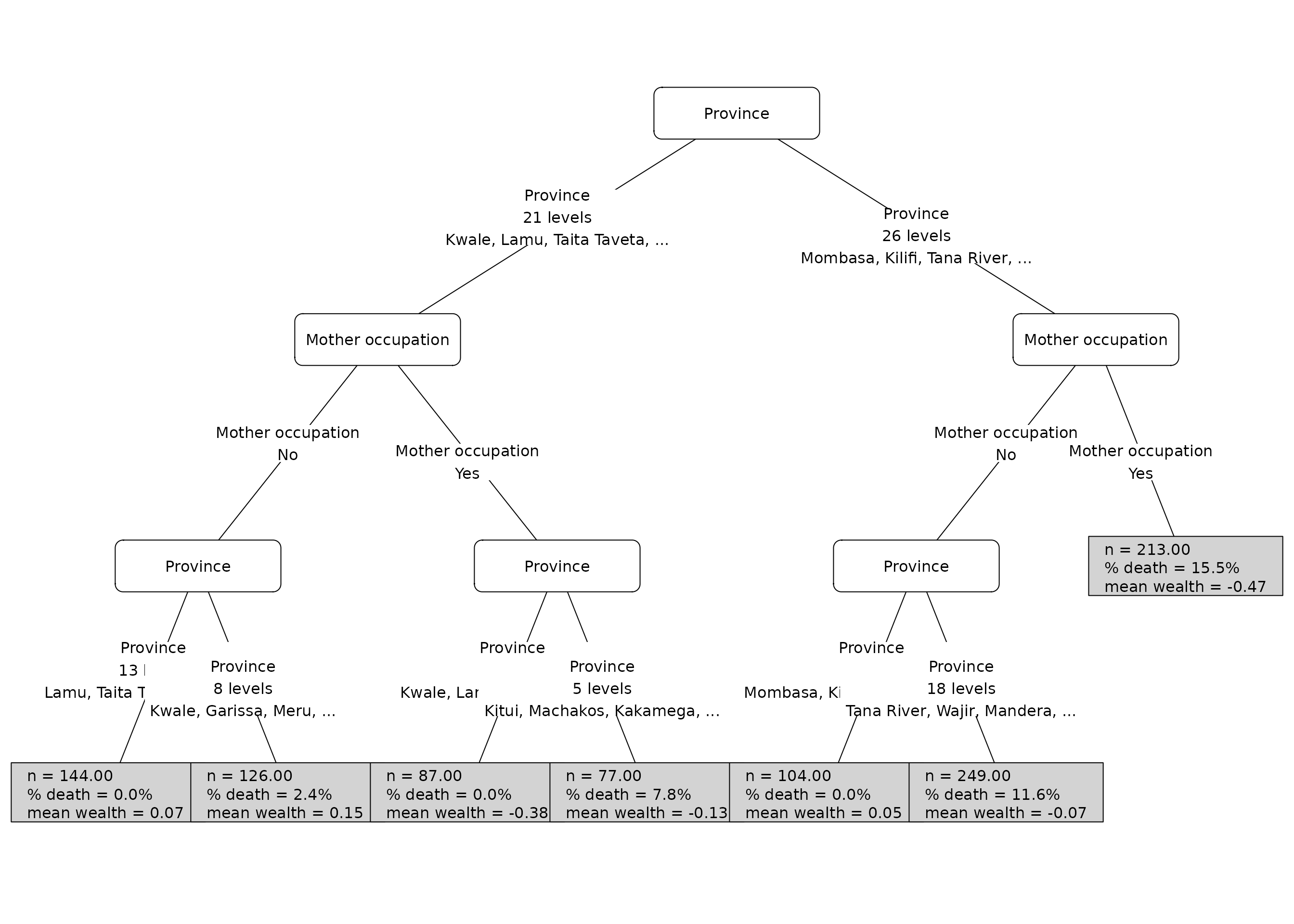
With those arguments, the terminal panels become self-contained: a reader can see not only where the split sends observations, but also how large each group is, how common under-five death is in the group, and where the group sits on the wealth ranking.
6. Use the tree as a prediction rule
The tree is fitted to explain inequality, but it can also be used as a simple risk model by assigning each child the mean outcome in their terminal node.
tree_risk <- predict_ci_tree_terminal_mean(
  fit = tree_fit,
  train_data = kenya_model,
  outcome_name = "deadu5_num",
  weights = kenya_model$sample_weight
)

kenya_model[
  ,
  .(
    observed_mortality = mean(deadu5_num),
    mean_tree_risk = mean(tree_risk)
  )
]
#>    observed_mortality mean_tree_risk
#>                 <num>          <num>
#> 1:              0.071     0.06702193
The validation-gain score asks whether the fitted partition reduces concentration-index impurity when observations are assigned to terminal nodes.
ci_tree_validation_gain(
  fit = tree_fit,
  new_data = kenya_model,
  rank_name = "wealth",
  outcome_name = "deadu5_num",
  weights = kenya_model$sample_weight
)
#> [1] 0.2087216
7. Select a tree by cross-validation
Tree depth, minimum node size, and the concentration-index objective
all control the trade-off between detail and stability.
tune_ci_tree() is the model-selection helper: it evaluates
candidate controls by cross-validation, scores each candidate on
held-out folds, and can refit the selected tree on the full analysis
table.
The default metric is "validation_gain", which selects
the model that most reduces concentration-index impurity on validation
folds. Prediction-oriented metrics are also available with
metric = "brier", "log_loss", or
"roc_auc". The relative gain metric scales validation gain
by the fold’s root impurity, which is useful when comparing
concentration-index criteria. The example below keeps the grid small so
the vignette builds quickly.
tuning_grid <- ci_tree_control_grid(
  minsplit = c(120L, 180L),
  minbucket = c(60L),
  minprob = 0.05,
  maxdepth = 2:3
)

tree_tuning <- tune_ci_tree(
  formula = cbind(wealth, deadu5_num) ~ rural + ed + reg + unskilled,
  data = kenya_model,
  rank_name = "wealth",
  outcome_name = "deadu5_num",
  weights = kenya_model$sample_weight,
  type = criterion_types,
  control_grid = tuning_grid,
  v = 3L,
  strata = "deadu5_num",
  seed = 20260512,
  metrics = c("validation_gain", "relative_validation_gain"),
  refit = TRUE
)

tree_tuning_metrics <- ci_collect_metrics(
  tree_tuning,
  metric = c("validation_gain", "relative_validation_gain"),
  format = "wide"
)

tree_tuning_metrics[
  order(-mean_validation_gain),
  .(
    type,
    minsplit,
    minbucket,
    maxdepth,
    mean_validation_gain,
    mean_validation_relative_gain
  )
]
#>       type minsplit minbucket maxdepth mean_validation_gain
#>     <char>    <int>     <int>    <int>                <num>
#>  1:      L      120        60        2          0.132214815
#>  2:      L      180        60        2          0.131636719
#>  3:      L      120        60        3          0.128289222
#>  4:      L      180        60        3          0.128153774
#>  5:    CIc      120        60        2          0.008560267
#>  6:    CIc      180        60        2          0.008038443
#>  7:    CIg      120        60        2          0.002140067
#>  8:    CIg      180        60        2          0.002009611
#>  9:    CIg      120        60        3         -0.003316367
#> 10:    CIg      180        60        3         -0.003446823
#> 11:    CIc      120        60        3         -0.013265468
#> 12:    CIc      180        60        3         -0.013787293
#> 13:     CI      120        60        3         -0.103124833
#> 14:     CI      120        60        2         -0.106396559
#> 15:     CI      180        60        2         -0.106396559
#> 16:     CI      180        60        3         -0.124843924
#>     mean_validation_relative_gain
#>                             <num>
#>  1:                    0.59288604
#>  2:                    0.58642506
#>  3:                    0.57576127
#>  4:                    0.57760310
#>  5:                    0.02317466
#>  6:                    0.01260733
#>  7:                    0.02317466
#>  8:                    0.01260733
#>  9:                   -0.55993363
#> 10:                   -0.57050096
#> 11:                   -0.55993363
#> 12:                   -0.57050096
#> 13:                   -0.68949870
#> 14:                   -0.66753594
#> 15:                   -0.66753594
#> 16:                   -0.72176091
The tuning object stores fold-level metrics, grid-level summaries, selected controls, and optional diagnostics. The collector helpers give a stable way to inspect those pieces without relying on list internals.
tree_selected <- ci_select_best(tree_tuning, metric = "validation_gain")

ci_fit_summary_table(
  tree_tuning,
  selected = tree_selected,
  metrics = c(
    "train_gain",
    "validation_gain",
    "train_relative_gain",
    "relative_validation_gain"
  )
)[
  ,
  .(
    type,
    minsplit,
    minbucket,
    maxdepth,
    mean_root_objective,
    mean_train_gain,
    mean_validation_gain,
    mean_validation_relative_gain,
    mean_percent_validation_gain
  )
]
#>      type minsplit minbucket maxdepth mean_root_objective mean_train_gain
#>    <char>    <int>     <int>    <int>               <num>           <num>
#> 1:     CI      120        60        3          0.34607946      0.22135164
#> 2:    CIc      120        60        2          0.10462579      0.04966298
#> 3:    CIg      120        60        2          0.02615645      0.01241574
#> 4:      L      120        60        2          0.20723936      0.17857896
#>    mean_validation_gain mean_validation_relative_gain
#>                   <num>                         <num>
#> 1:         -0.103124833                   -0.68949870
#> 2:          0.008560267                    0.02317466
#> 3:          0.002140067                    0.02317466
#> 4:          0.132214815                    0.59288604
#>    mean_percent_validation_gain
#>                           <num>
#> 1:                   -29.798022
#> 2:                     8.181794
#> 3:                     8.181794
#> 4:                    63.798120

tree_selected[
  ,
  .(type, minsplit, minbucket, maxdepth)
]
#>      type minsplit minbucket maxdepth
#>    <char>    <int>     <int>    <int>
#> 1:     CI      120        60        3
#> 2:    CIg      120        60        2
#> 3:    CIc      120        60        2
#> 4:      L      120        60        2
control_ci_tune() controls optional outputs. Here we
score two metrics in a single cross-validation run, save validation
predictions, and extract a small diagnostic from each fitted fold-level
tree.
diagnostic_tuning <- tune_ci_tree(
  formula = cbind(wealth, deadu5_num) ~ rural + ed + reg + unskilled,
  data = kenya_model,
  rank_name = "wealth",
  outcome_name = "deadu5_num",
  weights = kenya_model$sample_weight,
  type = "CI",
  control_grid = tuning_grid[1],
  v = 2L,
  strata = "deadu5_num",
  seed = 20260514,
  metrics = c("validation_gain", "brier"),
  control = control_ci_tune(
    save_pred = TRUE,
    extract = function(fit) {
      length(partykit::nodeids(fit, terminal = TRUE))
    }
  ),
  refit = FALSE
)

ci_collect_metrics(diagnostic_tuning, format = "wide")[
  ,
  .(
    type,
    mean_validation_gain,
    std_err_validation_gain,
    mean_brier,
    std_err_brier
  )
]
#>      type mean_validation_gain std_err_validation_gain mean_brier std_err_brier
#>    <char>                <num>                   <num>      <num>         <num>
#> 1:     CI          -0.05732995              0.01278988 0.06954765   0.002500993

head(ci_collect_predictions(diagnostic_tuning)[
  ,
  .(grid_id, fold_id, row_id, outcome, .pred)
])
#>    grid_id fold_id row_id outcome       .pred
#>      <int>   <int>  <int>   <num>       <num>
#> 1:       1       1      2       0 0.284437410
#> 2:       1       1      6       0 0.008842424
#> 3:       1       1      8       0 0.058991833
#> 4:       1       1      9       0 0.008842424
#> 5:       1       1     10       0 0.126348589
#> 6:       1       1     12       0 0.126348589

ci_collect_extracts(diagnostic_tuning)[
  ,
  .(
    grid_id,
    fold_id,
    type,
    terminal_nodes = unlist(.extracts)
  )
]
#>    grid_id fold_id   type terminal_nodes
#>      <int>   <int> <char>          <int>
#> 1:       1       1     CI              4
#> 2:       1       2     CI              3
When you already use rsample, you can pass an rset with
resamples instead of asking ineqTrees to
create folds from v and strata.
if (requireNamespace("rsample", quietly = TRUE)) {
  tree_folds <- rsample::vfold_cv(
    as.data.frame(kenya_model),
    v = 2L,
    strata = deadu5_num
  )

  rsample_tuning <- tune_ci_tree(
    formula = cbind(wealth, deadu5_num) ~ rural + ed + reg + unskilled,
    data = kenya_model,
    rank_name = "wealth",
    outcome_name = "deadu5_num",
    weights = kenya_model$sample_weight,
    type = "CI",
    control_grid = tuning_grid[1],
    resamples = tree_folds,
    seed = 20260515,
    refit = FALSE
  )

  ci_collect_metrics(rsample_tuning, format = "wide")[
    ,
    .(type, mean_validation_gain, n_validation_gain)
  ]
}
#>      type mean_validation_gain n_validation_gain
#>    <char>                <num>             <int>
#> 1:     CI          -0.02424206                 2
The top rows show the best candidates across the whole tuning run. Because the four criteria are on different numerical scales, it is also useful to report the best setting within each criterion and scale the validation gain by that criterion’s root impurity.
tree_best_by_type <- ci_select_best(
  tree_tuning,
  metric = "relative_validation_gain"
)

tree_best_by_type_table <- ci_fit_summary_table(
  tree_tuning,
  selected = tree_best_by_type,
  metrics = c(
    "train_gain",
    "validation_gain",
    "train_relative_gain",
    "relative_validation_gain"
  )
)[
  ,
  .(
    type,
    minsplit,
    minbucket,
    minprob,
    maxdepth,
    mean_root_objective,
    mean_train_gain,
    mean_validation_gain,
    mean_validation_relative_gain,
    mean_percent_validation_gain
  )
]

tree_best_by_type_table[
  ,
  mean_percent_validation_gain := sprintf("%.1f%%", mean_percent_validation_gain)
]

tree_best_by_type_table
#>      type minsplit minbucket minprob maxdepth mean_root_objective
#>    <char>    <int>     <int>   <num>    <int>               <num>
#> 1:     CI      120        60    0.05        2          0.34607946
#> 2:    CIc      120        60    0.05        2          0.10462579
#> 3:    CIg      120        60    0.05        2          0.02615645
#> 4:      L      120        60    0.05        2          0.20723936
#>    mean_train_gain mean_validation_gain mean_validation_relative_gain
#>              <num>                <num>                         <num>
#> 1:      0.19193408         -0.106396559                   -0.66753594
#> 2:      0.04966298          0.008560267                    0.02317466
#> 3:      0.01241574          0.002140067                    0.02317466
#> 4:      0.17857896          0.132214815                    0.59288604
#>    mean_percent_validation_gain
#>                          <char>
#> 1:                       -30.7%
#> 2:                         8.2%
#> 3:                         8.2%
#> 4:                        63.8%
The selected tree is available as tree_tuning$best_fit,
and the selected index is available as
tree_tuning$best_type. The best fit can be printed,
summarized, or plotted in the same way as tree_fit.
tree_tuning$best_params[
  ,
  .(type, minsplit, minbucket, maxdepth)
]
#>      type minsplit minbucket maxdepth
#>    <char>    <int>     <int>    <int>
#> 1:     CI      120        60        3
#> 2:    CIg      120        60        2
#> 3:    CIc      120        60        2
#> 4:      L      120        60        2
8. Fit and tune a concentration-index forest
ci_forest() averages predictions from many greedy
concentration-index trees. The forest can be useful when the goal is a
smoother risk estimate, while a surrogate tree can still be fitted
afterward for interpretation.
set.seed(20260512)

forest_fit <- ci_forest(
  formula = cbind(wealth, deadu5_num) ~ rural + ed + reg + unskilled,
  data = kenya_model,
  rank_name = "wealth",
  outcome_name = "deadu5_num",
  weights = kenya_model$sample_weight,
  ntree = 20L,
  mtry = 2L,
  control = ci_tree_control(
    minsplit = 120,
    minbucket = 60,
    minprob = 0.05,
    maxdepth = 3
  )
)

ci_forest_summary(forest_fit)
#>    ntree  mtry   type     n mean_outcome mean_prediction outcome_ci
#>    <int> <int> <char> <int>        <num>           <num>      <num>
#> 1:    20     2     CI  1000   0.06790072      0.06913558  0.3676449
#>    prediction_ci mean_terminal_nodes mean_max_depth
#>            <num>               <num>          <num>
#> 1:    0.09112755                 3.5            2.2
ci_forest_surrogate() fits an interpretable greedy tree
to the fitted forest predictions. Forest tuning still returns a
surrogate for interpretation, while the forest validation-gain metric
itself is computed from the forest’s stored member trees.
forest_surrogate <- ci_forest_surrogate(
  forest_fit,
  data = kenya_model,
  formula = cbind(wealth, deadu5_num) ~ rural + ed + reg + unskilled,
  rank_name = "wealth",
  weights = kenya_model$sample_weight,
  prediction_name = "forest_risk",
  control = ci_tree_control(
    minsplit = 120,
    minbucket = 60,
    minprob = 0.05,
    maxdepth = 2
  )
)

ci_tree_terminal_summary(forest_surrogate$fit)[
  ,
  .(node, n, depth, outcome_percent, rule)
]
#>     node     n depth outcome_percent
#>    <int> <int> <int>           <num>
#> 1:     3   201     2        4.472907
#> 2:     4   570     2        5.998426
#> 3:     6   137     2       10.408561
#> 4:     7    92     2       13.869669
#>                                                                                                                                                                                                                                                                                                                                                                                 rule
#>                                                                                                                                                                                                                                                                                                                                                                               <char>
#> 1: reg in {Mombasa, Kwale, Tana River, Lamu, Taita Taveta, Garissa, Isiolo, Meru, Tharaka-Nithi, Embu, Kitui, Machakos, Makueni, Nyandarua, Nyeri, Kirinyaga, Murang'a, Kiambu, Samburu, Trans Nzoia, Uasin Gishu, Elgeyo-Marakwet, Baringo, Laikipia, Narok, Kajiado, Kericho, Bomet, Kakamega, Vihiga, Bungoma, Busia, Kisumu, Migori, Kisii, Nyamira, Nairobi} & rural in {Urban}
#> 2: reg in {Mombasa, Kwale, Tana River, Lamu, Taita Taveta, Garissa, Isiolo, Meru, Tharaka-Nithi, Embu, Kitui, Machakos, Makueni, Nyandarua, Nyeri, Kirinyaga, Murang'a, Kiambu, Samburu, Trans Nzoia, Uasin Gishu, Elgeyo-Marakwet, Baringo, Laikipia, Narok, Kajiado, Kericho, Bomet, Kakamega, Vihiga, Bungoma, Busia, Kisumu, Migori, Kisii, Nyamira, Nairobi} & rural in {Rural}
#> 3:                                                                                                                                                                                                                                                                reg in {Kilifi, Wajir, Mandera, Marsabit, Turkana, West Pokot, Nandi, Nakuru, Siaya, Homa Bay} & unskilled in {No}
#> 4:                                                                                                                                                                                                                                                               reg in {Kilifi, Wajir, Mandera, Marsabit, Turkana, West Pokot, Nandi, Nakuru, Siaya, Homa Bay} & unskilled in {Yes}
The same cross-validation idea applies to forests.
tune_ci_forest() tunes forest controls and computes
validation gain by averaging the held-out concentration-index gain
across the forest’s internal tree partitions. Prediction metrics are
computed from the averaged forest predictions, and the selected refit
still includes an interpretable surrogate tree. The grid below uses
dials to create a regular search over familiar tidymodels
parameters, then converts the result with ci_dials_grid().
For a larger applied analysis, you could use levels = 3L or
add dials::tree_depth() and dials::trees() to
the grid.
forest_dials_grid <- dials::grid_regular(
  dials::mtry(range = c(2L, length(predictors))),
  dials::min_n(range = c(60L, 120L)),
  levels = 2L
)

forest_grid <- ci_dials_grid(
  forest_dials_grid,
  minprob = 0.05,
  maxdepth = 2L,
  ntree = 8L
)

forest_tuning <- tune_ci_forest(
  formula = cbind(wealth, deadu5_num) ~ rural + ed + reg + unskilled,
  data = kenya_model,
  rank_name = "wealth",
  outcome_name = "deadu5_num",
  weights = kenya_model$sample_weight,
  type = criterion_types,
  control_grid = forest_grid,
  v = 3L,
  strata = "deadu5_num",
  seed = 20260513,
  metrics = c("validation_gain", "relative_validation_gain", "brier"),
  control = control_ci_tune(save_pred = TRUE),
  refit = TRUE
)

forest_best_by_type <- ci_select_best(
  forest_tuning,
  metric = "relative_validation_gain"
)

forest_best_by_type_table <- ci_fit_summary_table(
  forest_tuning,
  selected = forest_best_by_type,
  metrics = c(
    "train_gain",
    "validation_gain",
    "train_relative_gain",
    "relative_validation_gain"
  )
)[
  ,
  .(
    type,
    ntree,
    mtry,
    minsplit,
    minbucket,
    minprob,
    maxdepth,
    mean_root_objective,
    mean_train_gain,
    mean_validation_gain,
    mean_validation_relative_gain,
    mean_percent_validation_gain
  )
]

forest_best_by_type_table[
  ,
  mean_percent_validation_gain := sprintf("%.1f%%", mean_percent_validation_gain)
]

forest_best_by_type_table
#>      type ntree  mtry minsplit minbucket minprob maxdepth mean_root_objective
#>    <char> <int> <int>    <int>     <int>   <num>    <int>               <num>
#> 1:     CI     8     2      120        60    0.05        2          0.38769935
#> 2:    CIc     8     2      240       120    0.05        2          0.10312638
#> 3:    CIg     8     2      240       120    0.05        2          0.02578159
#> 4:      L     8     4      120        60    0.05        2          0.22406928
#>    mean_train_gain mean_validation_gain mean_validation_relative_gain
#>              <num>                <num>                         <num>
#> 1:     0.016162851         -0.032299629                    -0.5924051
#> 2:     0.006035299         -0.005042323                    -0.4201404
#> 3:     0.001581413         -0.001453106                    -0.5233904
#> 4:     0.155144484          0.143722680                     0.6358682
#>    mean_percent_validation_gain
#>                          <char>
#> 1:                        -8.3%
#> 2:                        -4.9%
#> 3:                        -5.6%
#> 4:                        64.1%
The same collector helpers work for forests. With
save_pred = TRUE, the validation predictions are available
for quick diagnostic checks.
ci_fit_summary_table(
  forest_tuning,
  selected = forest_best_by_type,
  metrics = c(
    "train_gain",
    "validation_gain",
    "train_relative_gain",
    "relative_validation_gain"
  )
)[
  ,
  .(
    type,
    ntree,
    mtry,
    minbucket,
    mean_validation_gain,
    mean_percent_validation_gain
  )
]
#>      type ntree  mtry minbucket mean_validation_gain
#>    <char> <int> <int>     <int>                <num>
#> 1:     CI     8     2        60         -0.032299629
#> 2:    CIc     8     2       120         -0.005042323
#> 3:    CIg     8     2       120         -0.001453106
#> 4:      L     8     4        60          0.143722680
#>    mean_percent_validation_gain
#>                           <num>
#> 1:                    -8.331102
#> 2:                    -4.889460
#> 3:                    -5.636214
#> 4:                    64.142073

ci_collect_metrics(forest_tuning, metric = "brier", format = "wide")[
  order(mean_brier),
  .(type, ntree, mtry, mean_brier, std_err_brier)
]
#>       type ntree  mtry mean_brier std_err_brier
#>     <char> <int> <int>      <num>         <num>
#>  1:    CIg     8     2 0.06282187   0.004728063
#>  2:    CIc     8     2 0.06282860   0.005098547
#>  3:    CIc     8     2 0.06350273   0.005536247
#>  4:    CIg     8     2 0.06366306   0.005459293
#>  5:      L     8     2 0.06368060   0.005834791
#>  6:      L     8     2 0.06399172   0.005332748
#>  7:      L     8     4 0.06424526   0.005057308
#>  8:    CIc     8     4 0.06453011   0.004646087
#>  9:     CI     8     2 0.06453210   0.005098101
#> 10:    CIg     8     4 0.06454203   0.005354527
#> 11:     CI     8     4 0.06531002   0.006083495
#> 12:     CI     8     2 0.06542156   0.005173032
#> 13:      L     8     4 0.06553168   0.005348346
#> 14:    CIg     8     4 0.06703871   0.005694440
#> 15:    CIc     8     4 0.06785901   0.007002403
#> 16:     CI     8     4 0.06818806   0.005893820

head(ci_collect_predictions(forest_tuning)[
  ,
  .(grid_id, fold_id, type, row_id, outcome, .pred)
])
#>    grid_id fold_id   type row_id outcome      .pred
#>      <int>   <int> <char>  <int>   <num>      <num>
#> 1:       1       1     CI      4       0 0.07101437
#> 2:       1       1     CI      5       0 0.05645208
#> 3:       1       1     CI      7       0 0.04814214
#> 4:       1       1     CI     11       0 0.10638212
#> 5:       1       1     CI     12       0 0.07448763
#> 6:       1       1     CI     13       0 0.10518186
The percentage gain is calculated as
100 * mean_validation_gain / abs(mean_root_objective). This
shows how much of the validation-fold root concentration-index impurity
is recovered by the selected model for each concentration-index
criterion. Because the denominator is criterion-specific, the percentage
makes the gains easier to compare within each CI definition.
The fitted values are predicted risks. Their concentration index can be compared with the concentration index of the observed outcome.
9. Decompose fitted inequality with SHAP values
When model explanations are available as SHAP values,
shap_conc_decomp() decomposes the concentration index of
the fitted risk into feature-level contributions. This step is
model-agnostic: the SHAP values may come from an ineqTrees
forest, ranger, xgboost, or another prediction
model.
The small example below uses an already-aligned SHAP-style contribution table. In an applied workflow, this object would usually be produced by a SHAP package.
shap_example <- data.frame(
  residence = as.numeric(kenya_model$rural == "Rural") * 0.01,
  education = as.numeric(kenya_model$ed == "b no education") * 0.015,
  occupation = as.numeric(kenya_model$unskilled == "Yes") * 0.01
)

prediction <- mean(forest_risk) + rowSums(shap_example)

decomp <- shap_conc_decomp(
  shap = shap_example,
  rank = kenya_model$wealth,
  prediction = prediction,
  weights = kenya_model$sample_weight
)

decomp$contributions[
  order(-abs_contribution),
  .(feature, D_k_SHAP, pct_contribution)
]
#>       feature    D_k_SHAP pct_contribution
#>        <char>       <num>            <num>
#> 1:  education 0.013860108         43.93448
#> 2:  residence 0.011886472         37.67834
#> 3: occupation 0.005800644         18.38718
This decomposition should be read as a model-based explanation of fitted inequality, not as a causal attribution.
10. Where to go next
The introductory workflow covers the main objects:
-
ci_factory()for concentration-index scoring; -
ci_tree()for interpretable inequality-aware subgrouping withtype = "CI","CIg","CIc", or"L"; -
tune_ci_tree()for cross-validated model selection across tree controls and concentration-index objectives; -
control_ci_tune()and theci_collect_*()helpers for saving predictions, extracting fold diagnostics, collecting notes, and inspecting tuning results; -
ci_forest()for ensemble risk estimation; -
ci_forest_surrogate()for fitting an interpretable tree to forest predictions; -
ci_fit_summary_table()for report-ready tuning summaries; -
shap_conc_decomp()for decomposing fitted inequality when SHAP values are available.
The reference pages document the lower-level split-search helpers and plotting customization functions. Most analyses can start with the workflow shown here.