Shapley decomposition

library(ineqTrees)

Introduction

This article shows how SHAP values can be connected to the concentration-index decomposition in ineqTrees. The key point is model-agnostic: shap_conc_decomp() only needs SHAP values, a socioeconomic rank, and model predictions. Those predictions can come from an inequality-aware tree, an inequality-aware forest fitted through tidymodels, or an ordinary prediction model such as a ranger random forest.

The examples use the simulated Kenya child-survival data shipped with the package. We fit three models:

• a package-native ci_tree() and ci_forest();
• a tidymodels rand_forest(engine = "ineqTrees");
• a standard ranger forest for predicting under-five mortality.

Then we approximate SHAP values with shapr::explain(), decompose the concentration index of the fitted risks, and plot the feature contributions.

library(ineqTrees)
library(data.table)
#> 
#> Attaching package: 'data.table'
#> The following object is masked from 'package:base':
#> 
#>     %notin%
library(parsnip)
library(workflows)
library(rsample)
library(dials)
#> Loading required package: scales
library(tune)
library(yardstick)
library(hardhat)
library(shapr)
#> 
#> Attaching package: 'shapr'
#> The following object is masked from 'package:parsnip':
#> 
#>     prepare_data

register_ineqtrees_parsnip()

data(kenya, package = "ineqTrees")
setDT(kenya)

1. Prepare the analysis table

This chunk keeps the rank, outcome, predictors, and sample weight together. The same table is used for the inequality-aware models and for the ordinary prediction forest.

shap_predictors <- c("rural", "ed", "reg", "unskilled")

analysis_vars <- c(
  "wealth",
  "deadu5_num",
  shap_predictors,
  "sample_weight"
)

kenya_child <- kenya[
  complete.cases(kenya[, ..analysis_vars]),
  ..analysis_vars
]

set.seed(20260517)
kenya_model <- as.data.frame(
  kenya_child[sample.int(.N, min(800L, .N))]
)

kenya_model$case_wt <- hardhat::importance_weights(kenya_model$sample_weight)

model_x <- kenya_model[, shap_predictors, drop = FALSE]

eval_n <- min(250L, nrow(kenya_model))
eval_rows <- sort(sample.int(nrow(kenya_model), eval_n))
model_x_eval <- model_x[eval_rows, , drop = FALSE]
wealth_eval <- kenya_model$wealth[eval_rows]
weight_eval <- kenya_model$sample_weight[eval_rows]

head(kenya_model[, c("wealth", "deadu5_num", shap_predictors)])
#>       wealth deadu5_num rural             ed     reg unskilled
#> 1 -0.1604132          0 Rural    a education   Nyeri       Yes
#> 2  3.5337442          0 Urban    a education   Narok        No
#> 3 -0.2000321          0 Urban    a education  Migori       Yes
#> 4 -0.5770841          0 Rural    a education Samburu        No
#> 5 -0.4059414          0 Rural b no education   Narok        No
#> 6 -0.2732339          0 Rural    a education    Meru        No

2. Helper functions

This chunk defines prediction wrappers for shapr. Each wrapper accepts a model object and a predictor table, then returns one numeric risk for each row.

ci_tree_risk_predict <- function(object, newdata) {
  as.numeric(stats::predict(
    object,
    newdata = as.data.frame(newdata),
    type = "response"
  ))
}

ci_forest_risk_predict <- function(object, newdata) {
  as.numeric(stats::predict(
    object,
    newdata = as.data.frame(newdata),
    OOB = FALSE
  ))
}

ranger_risk_predict <- function(object, newdata) {
  prob <- predict(object, new_data = as.data.frame(newdata), type = "prob")
  as.numeric(prob$.pred_died)
}

extract_shapr_values <- function(explanation) {
  shap_values <- as.data.frame(explanation$shapley_values_est)
  shap_values[
    ,
    setdiff(names(shap_values), c("explain_id", "none")),
    drop = FALSE
  ]
}

estimate_shapr_values <- function(object,
                                  x_train,
                                  x_explain,
                                  pred_wrapper,
                                  seed,
                                  n_mc_samples = 32L) {
  model_specs <- function(unused) {
    list(
      labels = names(x_train),
      classes = vapply(x_train, function(col) class(col)[1], character(1)),
      factor_levels = lapply(x_train, function(col) {
        if (is.factor(col)) levels(col) else NULL
      })
    )
  }

  explanation <- shapr::explain(
    model = object,
    x_explain = as.data.frame(x_explain),
    x_train = as.data.frame(x_train),
    approach = "independence",
    phi0 = mean(pred_wrapper(object, x_train)),
    n_MC_samples = n_mc_samples,
    seed = seed,
    predict_model = pred_wrapper,
    get_model_specs = model_specs,
    verbose = NULL
  )

  extract_shapr_values(explanation)
}

plot_shap_contributions <- function(contributions, title) {

  ggplot2::ggplot(
    contributions,
    ggplot2::aes(
      x = stats::reorder(feature, pct_contribution),
      y = pct_contribution,
      fill = pct_contribution > 0
    )
  ) +
    ggplot2::geom_col(width = 0.7) +
    ggplot2::coord_flip() +
    ggplot2::scale_fill_manual(
      values = c("#2166ac", "#b2182b"),
      guide = "none"
    ) +
    ggplot2::labs(
      x = NULL,
      y = "Percentage contribution",
      title = title
    ) +
    ggplot2::theme_minimal(base_size = 12) +
    ggplot2::theme(panel.grid.minor = ggplot2::element_blank())
}

3. Fit package-native inequality-aware models

This chunk fits a single concentration-index tree and a small concentration-index forest with the package-native API. These models optimize concentration-index split gain, so they are explanatory subgrouping models first and prediction models second.

tree_fit <- ci_tree(
  formula = cbind(wealth, deadu5_num) ~ rural + ed + reg + unskilled,
  data = kenya_model,
  rank_name = "wealth",
  outcome_name = "deadu5_num",
  weights = kenya_model$sample_weight,
  type = "CI",
  control = ci_tree_control(
    minsplit = 120L,
    minbucket = 60L,
    minprob = 0.05,
    maxdepth = 3L
  )
)

set.seed(20260517)
forest_fit <- ci_forest(
  formula = cbind(wealth, deadu5_num) ~ rural + ed + reg + unskilled,
  data = kenya_model,
  rank_name = "wealth",
  outcome_name = "deadu5_num",
  weights = kenya_model$sample_weight,
  type = "CI",
  ntree = 20L,
  mtry = 2L,
  control = ci_tree_control(
    minsplit = 120L,
    minbucket = 60L,
    minprob = 0.05,
    maxdepth = 3L
  )
)

ci_forest_summary(forest_fit)
#>    ntree  mtry   type     n mean_outcome mean_prediction outcome_ci
#>    <int> <int> <char> <int>        <num>           <num>      <num>
#> 1:    20     2     CI   800    0.0840066      0.08094287  0.1777822
#>    prediction_ci mean_terminal_nodes mean_max_depth
#>            <num>               <num>          <num>
#> 1:     0.0766643                2.85            1.8

4. Decompose the inequality-aware tree

This chunk approximates SHAP values for the tree predictions and then decomposes the concentration index of those fitted risks.

set.seed(20260517)

tree_pred_eval <- ci_tree_risk_predict(tree_fit, model_x_eval)

tree_shap <- estimate_shapr_values(
  object = tree_fit,
  x_train = model_x,
  x_explain = model_x_eval,
  pred_wrapper = ci_tree_risk_predict,
  seed = 20260517
)

tree_decomp <- shap_conc_decomp(
  shap = tree_shap,
  rank = wealth_eval,
  prediction = tree_pred_eval,
  weights = weight_eval,
  type = "CI"
)

knitr::kable(
  as.data.frame(tree_decomp$diagnostics),
  digits = 3,
  caption = "CI tree SHAP decomposition diagnostics"
)

CI tree SHAP decomposition diagnostics

n	weight_sum	type	mean_prediction	concentration_index	signed_concentration_index	score_direction	shap_sum	additivity_gap	centered_rank_sum	prediction_source
250	207.353	CI	0.081	0.143	-0.143	-1	0.143	0	0	prediction

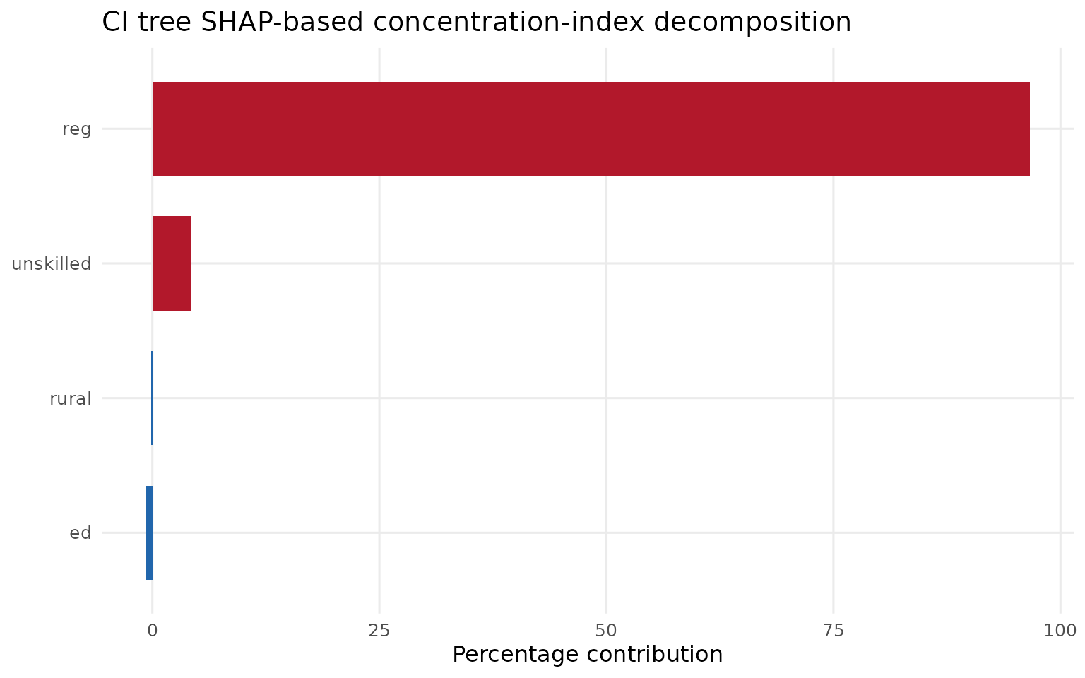
tree_contrib <- as.data.frame(tree_decomp$contributions)

knitr::kable(
  tree_contrib,
  digits = 3,
  caption = "CI tree SHAP-based concentration-index contributions"
)

CI tree SHAP-based concentration-index contributions

feature	D_k_SHAP	pct_contribution	abs_contribution
reg	0.138	96.596	0.138
unskilled	0.006	4.229	0.006
ed	-0.001	-0.697	0.001
rural	0.000	-0.129	0.000

plot_shap_contributions(
  tree_contrib,
  "CI tree SHAP-based concentration-index decomposition"
)

5. Decompose the inequality-aware forest

The same decomposition works for a forest. The only difference is the prediction wrapper: for ci_forest(), predictions are averaged across trees.

set.seed(20260518)

forest_pred_eval <- ci_forest_risk_predict(forest_fit, model_x_eval)

forest_shap <- estimate_shapr_values(
  object = forest_fit,
  x_train = model_x,
  x_explain = model_x_eval,
  pred_wrapper = ci_forest_risk_predict,
  seed = 20260518
)

forest_decomp <- shap_conc_decomp(
  shap = forest_shap,
  rank = wealth_eval,
  prediction = forest_pred_eval,
  weights = weight_eval,
  type = "CI"
)

knitr::kable(
  as.data.frame(forest_decomp$diagnostics),
  digits = 3,
  caption = "CI forest SHAP decomposition diagnostics"
)

CI forest SHAP decomposition diagnostics

n	weight_sum	type	mean_prediction	concentration_index	signed_concentration_index	score_direction	shap_sum	additivity_gap	centered_rank_sum	prediction_source
250	207.353	CI	0.078	0.089	-0.089	-1	0.089	0	0	prediction

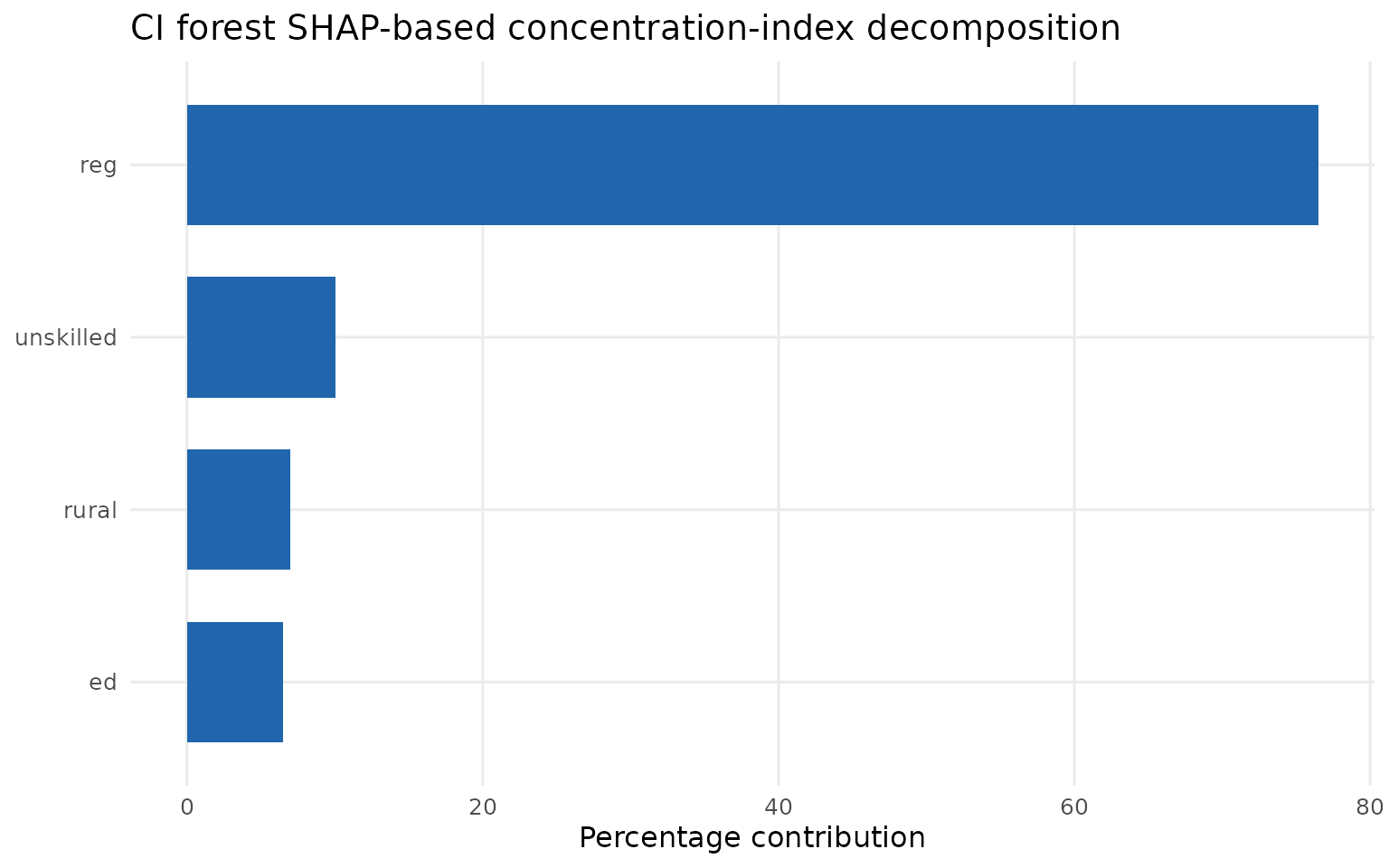
forest_contrib <- as.data.frame(forest_decomp$contributions)

knitr::kable(
  forest_contrib,
  digits = 3,
  caption = "CI forest SHAP-based concentration-index contributions"
)

CI forest SHAP-based concentration-index contributions

feature	D_k_SHAP	pct_contribution	abs_contribution
reg	0.068	76.472	0.068
unskilled	0.009	10.019	0.009
rural	0.006	7.003	0.006
ed	0.006	6.505	0.006

plot_shap_contributions(
  forest_contrib,
  "CI forest SHAP-based concentration-index decomposition"
)

6. Fit an inequality-aware forest with tidymodels

This chunk fits the same model family through parsnip and workflows. The formula includes wealth so the parsnip bridge has the rank column available; the bridge then removes wealth from the split predictors internally.

tidy_forest_spec <- rand_forest(
  trees = 20L,
  mtry = 2L,
  min_n = 60L
) |>
  set_engine(
    "ineqTrees",
    rank_name = "wealth",
    outcome_name = "deadu5_num",
    type = "CI",
    minsplit = 120L,
    minprob = 0.05,
    maxdepth = 3L
  ) |>
  set_mode("regression")

tidy_forest_wf <- workflow() |>
  add_model(tidy_forest_spec) |>
  add_formula(deadu5_num ~ wealth + rural + ed + reg + unskilled) |>
  add_case_weights(case_wt)

set.seed(20260519)
tidy_forest_fit <- fit(tidy_forest_wf, data = kenya_model)
tidy_forest_engine <- extract_fit_parsnip(tidy_forest_fit)$fit

ci_forest_summary(tidy_forest_engine)
#>    ntree  mtry   type     n mean_outcome mean_prediction outcome_ci
#>    <int> <int> <char> <int>        <num>           <num>      <num>
#> 1:    20     2     CI   800    0.0840066      0.08302601  0.1777822
#>    prediction_ci mean_terminal_nodes mean_max_depth
#>            <num>               <num>          <num>
#> 1:    0.06150863                 2.7            1.6

7. Decompose the tidymodels inequality-aware forest

The workflow formula includes wealth so the engine can learn inequality-aware splits. For SHAP, we explain the fitted engine extracted from the workflow, because the engine predicts from the split predictors without treating the rank column as a determinant.

set.seed(20260519)

tidy_forest_pred_eval <- ci_forest_risk_predict(
  tidy_forest_engine,
  model_x_eval
)

tidy_forest_shap <- estimate_shapr_values(
  object = tidy_forest_engine,
  x_train = model_x,
  x_explain = model_x_eval,
  pred_wrapper = ci_forest_risk_predict,
  seed = 20260519
)

tidy_forest_decomp <- shap_conc_decomp(
  shap = tidy_forest_shap,
  rank = wealth_eval,
  prediction = tidy_forest_pred_eval,
  weights = weight_eval,
  type = "CI"
)

knitr::kable(
  as.data.frame(tidy_forest_decomp$diagnostics),
  digits = 3,
  caption = "Tidymodels CI forest SHAP decomposition diagnostics"
)

Tidymodels CI forest SHAP decomposition diagnostics

n	weight_sum	type	mean_prediction	concentration_index	signed_concentration_index	score_direction	shap_sum	additivity_gap	centered_rank_sum	prediction_source
250	207.353	CI	0.08	0.076	-0.076	-1	0.076	0	0	prediction

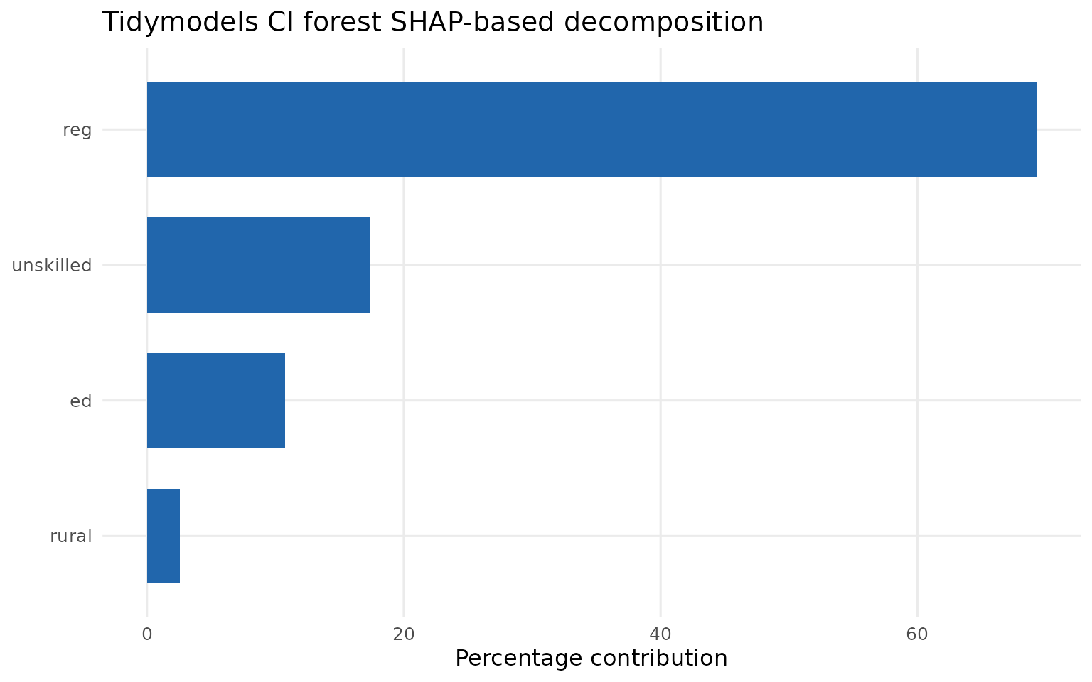
tidy_forest_contrib <- as.data.frame(tidy_forest_decomp$contributions)

plot_shap_contributions(
  tidy_forest_contrib,
  "Tidymodels CI forest SHAP-based decomposition"
)

8. Fit a prediction-focused ranger forest

The decomposition does not require an inequality-aware model. This chunk fits a standard ranger random forest whose target is prediction of under-five mortality. The model is classification-focused; the decomposition is applied afterward to the predicted mortality risk.

ranger_data <- kenya_model
ranger_data$deadu5 <- factor(
  ifelse(ranger_data$deadu5_num == 1, "died", "alive"),
  levels = c("died", "alive")
)

set.seed(20260520)
ranger_folds <- vfold_cv(ranger_data, v = 3L, strata = deadu5)

ranger_spec <- rand_forest(
  trees = 200L,
  mtry = tune(),
  min_n = tune()
) |>
  set_engine("ranger", probability = TRUE) |>
  set_mode("classification")

ranger_wf <- workflow() |>
  add_model(ranger_spec) |>
  add_formula(deadu5 ~ rural + ed + reg + unskilled)

ranger_grid <- grid_regular(
  mtry(range = c(1L, length(shap_predictors))),
  min_n(range = c(5L, 40L)),
  levels = 2L
)

set.seed(20260520)
ranger_tuned <- tune_grid(
  ranger_wf,
  resamples = ranger_folds,
  grid = ranger_grid,
  metrics = metric_set(roc_auc, accuracy)
)

best_ranger <- finalize_workflow(
  ranger_wf,
  select_best(ranger_tuned, metric = "roc_auc")
) |>
  fit(data = ranger_data)

collect_metrics(ranger_tuned)
#> # A tibble: 8 × 8
#>    mtry min_n .metric  .estimator  mean     n std_err .config        
#>   <int> <int> <chr>    <chr>      <dbl> <int>   <dbl> <chr>          
#> 1     1     5 accuracy binary     0.927     3  0.0165 pre0_mod1_post0
#> 2     1     5 roc_auc  binary     0.641     3  0.0336 pre0_mod1_post0
#> 3     1    40 accuracy binary     0.927     3  0.0165 pre0_mod2_post0
#> 4     1    40 roc_auc  binary     0.646     3  0.0349 pre0_mod2_post0
#> 5     4     5 accuracy binary     0.909     3  0.0120 pre0_mod3_post0
#> 6     4     5 roc_auc  binary     0.631     3  0.0340 pre0_mod3_post0
#> 7     4    40 accuracy binary     0.927     3  0.0165 pre0_mod4_post0
#> 8     4    40 roc_auc  binary     0.667     3  0.0247 pre0_mod4_post0

9. Decompose the ranger prediction model

This chunk explains the ordinary prediction model, then decomposes inequality in its predicted mortality risks. This is useful when the research question is: which predictors account for socioeconomic inequality in model-predicted mortality risk?

set.seed(20260521)

ranger_x <- ranger_data[, shap_predictors, drop = FALSE]
ranger_x_eval <- ranger_x[eval_rows, , drop = FALSE]
ranger_pred_eval <- ranger_risk_predict(best_ranger, ranger_x_eval)

ranger_shap <- estimate_shapr_values(
  object = best_ranger,
  x_train = ranger_x,
  x_explain = ranger_x_eval,
  pred_wrapper = ranger_risk_predict,
  seed = 20260521
)

ranger_decomp <- shap_conc_decomp(
  shap = ranger_shap,
  rank = ranger_data$wealth[eval_rows],
  prediction = ranger_pred_eval,
  weights = ranger_data$sample_weight[eval_rows],
  type = "CI"
)

knitr::kable(
  as.data.frame(ranger_decomp$diagnostics),
  digits = 3,
  caption = "Ranger SHAP decomposition diagnostics"
)

Ranger SHAP decomposition diagnostics

n	weight_sum	type	mean_prediction	concentration_index	signed_concentration_index	score_direction	shap_sum	additivity_gap	centered_rank_sum	prediction_source
250	207.353	CI	0.065	0.146	-0.146	-1	0.146	0	0	prediction

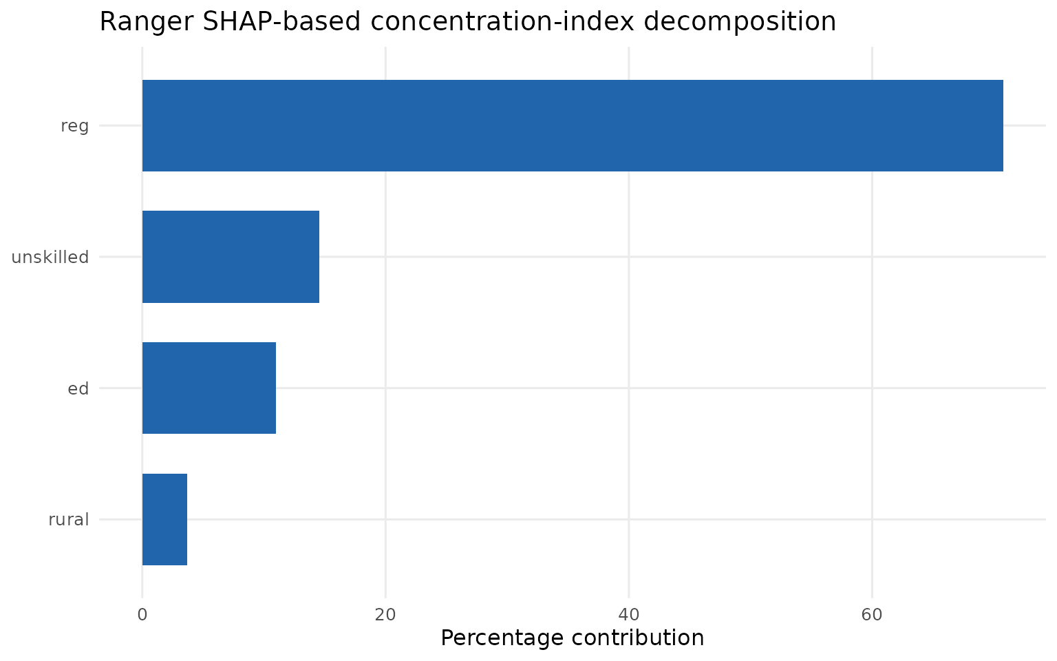
ranger_contrib <- as.data.frame(ranger_decomp$contributions)

knitr::kable(
  ranger_contrib,
  digits = 3,
  caption = "Ranger SHAP-based concentration-index contributions"
)

Ranger SHAP-based concentration-index contributions

feature	D_k_SHAP	pct_contribution	abs_contribution
reg	0.103	70.753	0.103
unskilled	0.021	14.560	0.021
ed	0.016	11.014	0.016
rural	0.005	3.673	0.005

plot_shap_contributions(
  ranger_contrib,
  "Ranger SHAP-based concentration-index decomposition"
)

10. Interpretation

The same decomposition table can be read for all three model families. Positive and negative contributions offset each other. The decomposition is model-based rather than causal: it explains inequality in the fitted predictions, not the causal effect of a determinant on mortality.

The important practical distinction is the model target:

• ci_tree() and ci_forest() build the inequality objective directly into the split search.
• rand_forest(engine = "ineqTrees") lets the same objective move through tidymodels workflows.
• rand_forest(engine = "ranger") is an ordinary mortality prediction model; shap_conc_decomp() then asks how its predicted risks are distributed across wealth.