Introduction
The fitted objects returned by ci_tree() inherit from
partykit tree objects, so the generic plot()
method works directly:
plot(tree)ineqTrees adds a plot.ci_tree() method on
top of the partykit layout. The method keeps the familiar
tree geometry while making the annotations more useful for
concentration-index trees:
- internal nodes show readable split-variable names;
- edge labels are compact, especially for factor splits with many levels;
- terminal nodes can show custom subgroup summaries;
- the same plot method works for ordinary fitted trees and forest surrogate trees.
This tutorial starts with the generic plot and then builds up the controls used most often in reports.
library(ineqTrees)
library(data.table)
#>
#> Attaching package: 'data.table'
#> The following object is masked from 'package:base':
#>
#>     %notin%
library(grid)

data(kenya, package = "ineqTrees")
setDT(kenya)

plot_vars <- c(
  "wealth",
  "deadu5_num",
  "rural",
  "ed",
  "reg",
  "unskilled",
  "sample_weight"
)

plot_data <- kenya[
  complete.cases(kenya[, ..plot_vars]),
  ..plot_vars
]

set.seed(20260521)
plot_data <- plot_data[
  sample.int(.N, min(900L, .N))
]

tree <- ci_tree(
  formula = cbind(wealth, deadu5_num) ~ rural + ed + reg + unskilled,
  data = plot_data,
  rank_name = "wealth",
  outcome_name = "deadu5_num",
  weights = plot_data$sample_weight,
  type = "CI",
  control = ci_tree_control(
    minsplit = 120,
    minbucket = 60,
    minprob = 0.05,
    maxdepth = 3
  )
)
Start With The Generic Plot
The simplest call is the one users already expect from an R model object:
plot(tree)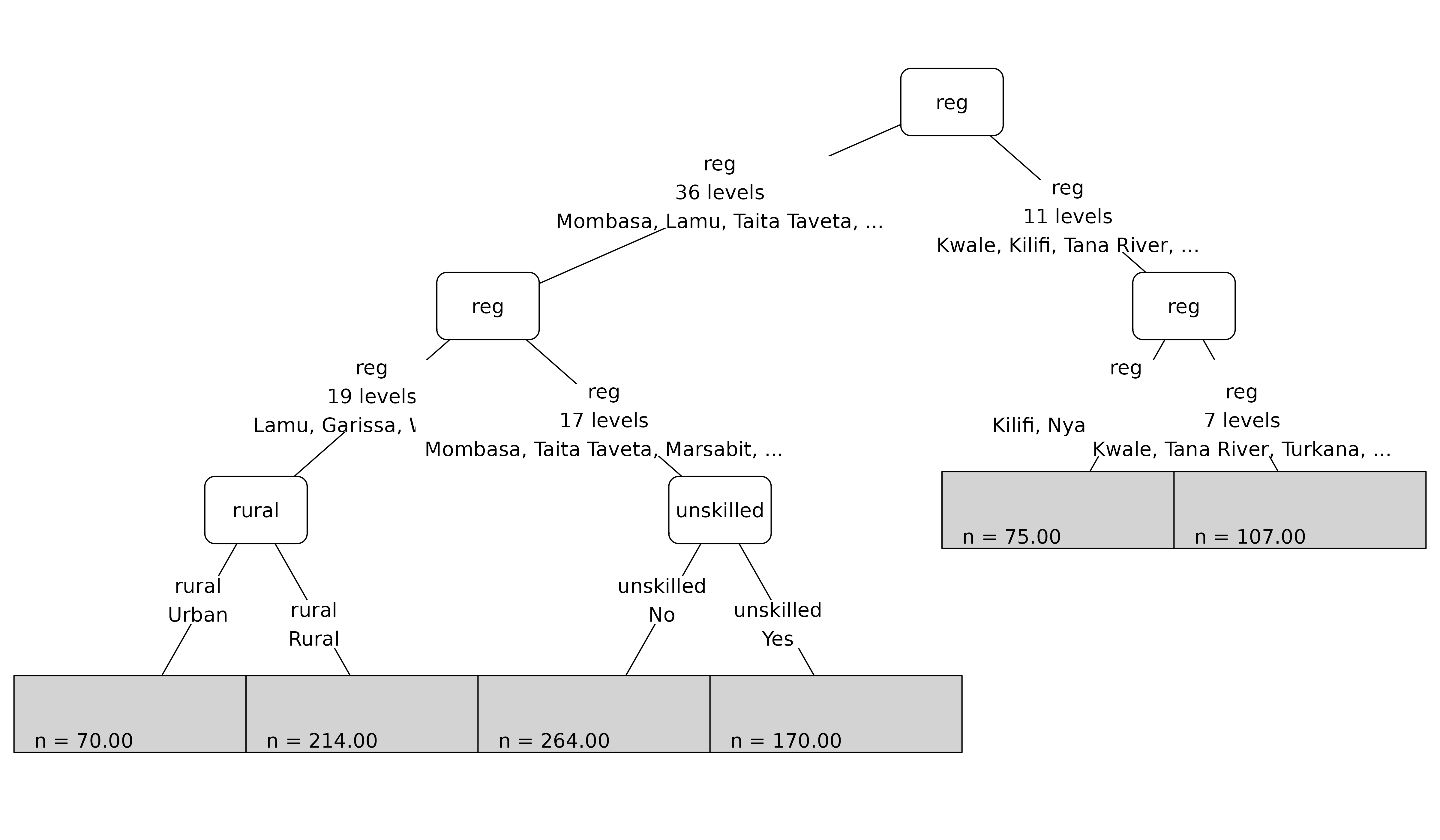
By default, the method draws compact split labels and terminal nodes with the number of observations in each terminal group. This is the fastest way to check whether the fitted tree has the shape you expected.
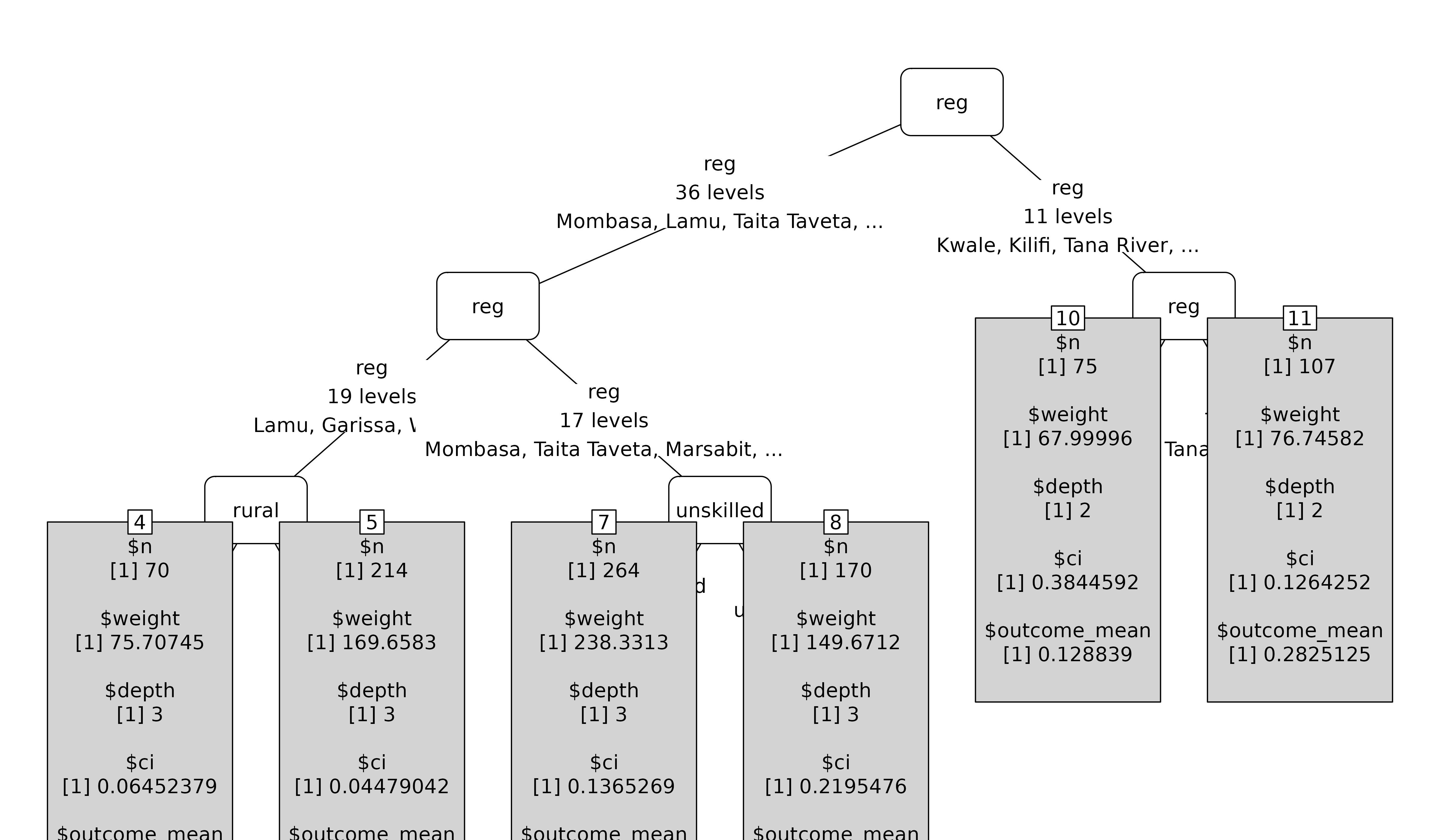
If you want the underlying partykit terminal-node panel
instead of the ineqTrees summary panel, set
terminal_stats = NULL.
plot(
  tree,
  terminal_stats = NULL
)
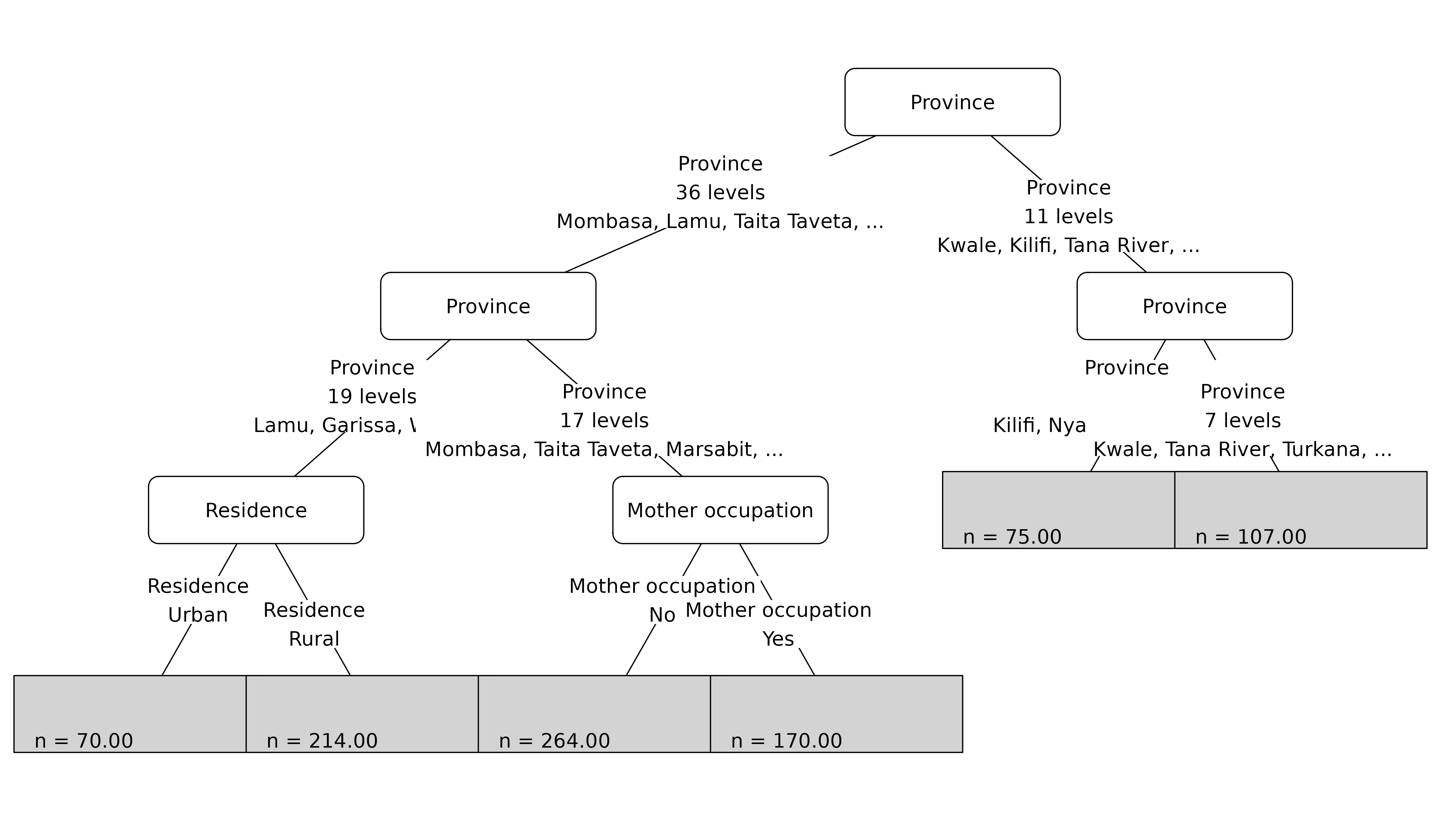
Use Readable Split Labels
The split variables in an analysis table often have short names. Use
var_labels to map those column names to report-ready
labels. The same labels are used in internal nodes and edge labels.
plot_labels <- c(
  rural = "Residence",
  ed = "Mother education",
  reg = "Province",
  unskilled = "Mother occupation"
)

plot(
  tree,
  var_labels = plot_labels
)
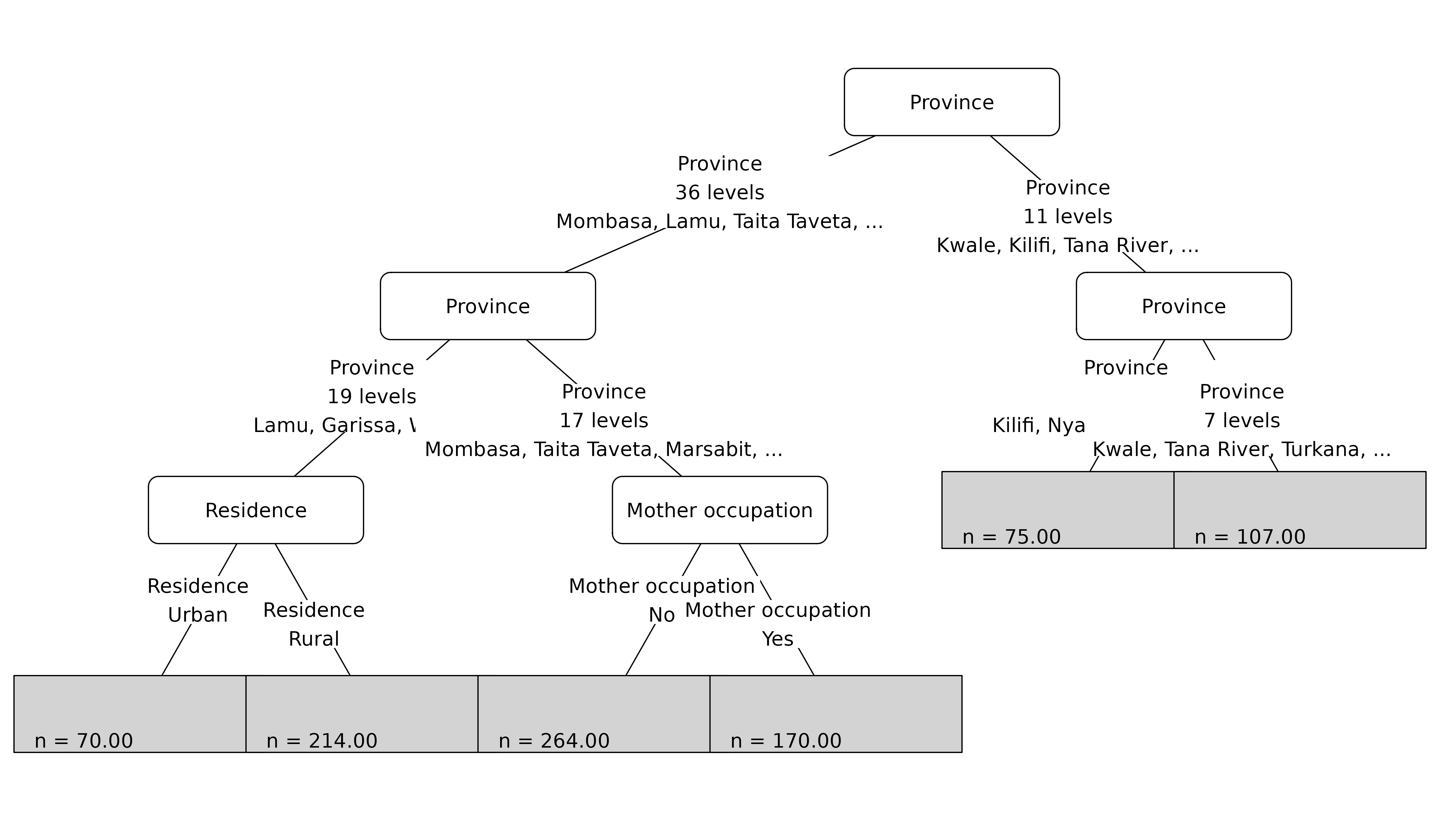
Factor splits can contain several levels on one side of a split. The
compact edge panel shortens long level lists automatically. When the
shortened label needs a domain-specific plural, use
plural_overrides.
Add Terminal-Node Statistics
For applied interpretation, the terminal nodes should usually show
the subgroup quantities you want readers to compare. Supply a named list
of functions through terminal_stats. Each function receives
the data assigned to one terminal node and must return one value.
node_stats <- list(
  n = nrow,
  mortality = function(df) mean(df$deadu5_num),
  mean_wealth = function(df) mean(df$wealth),
  weighted_n = function(df) sum(df$sample_weight)
)

plot(
  tree,
  data = plot_data,
  var_labels = plot_labels,
  plural_overrides = c(Province = "provinces"),
  terminal_stats = node_stats
)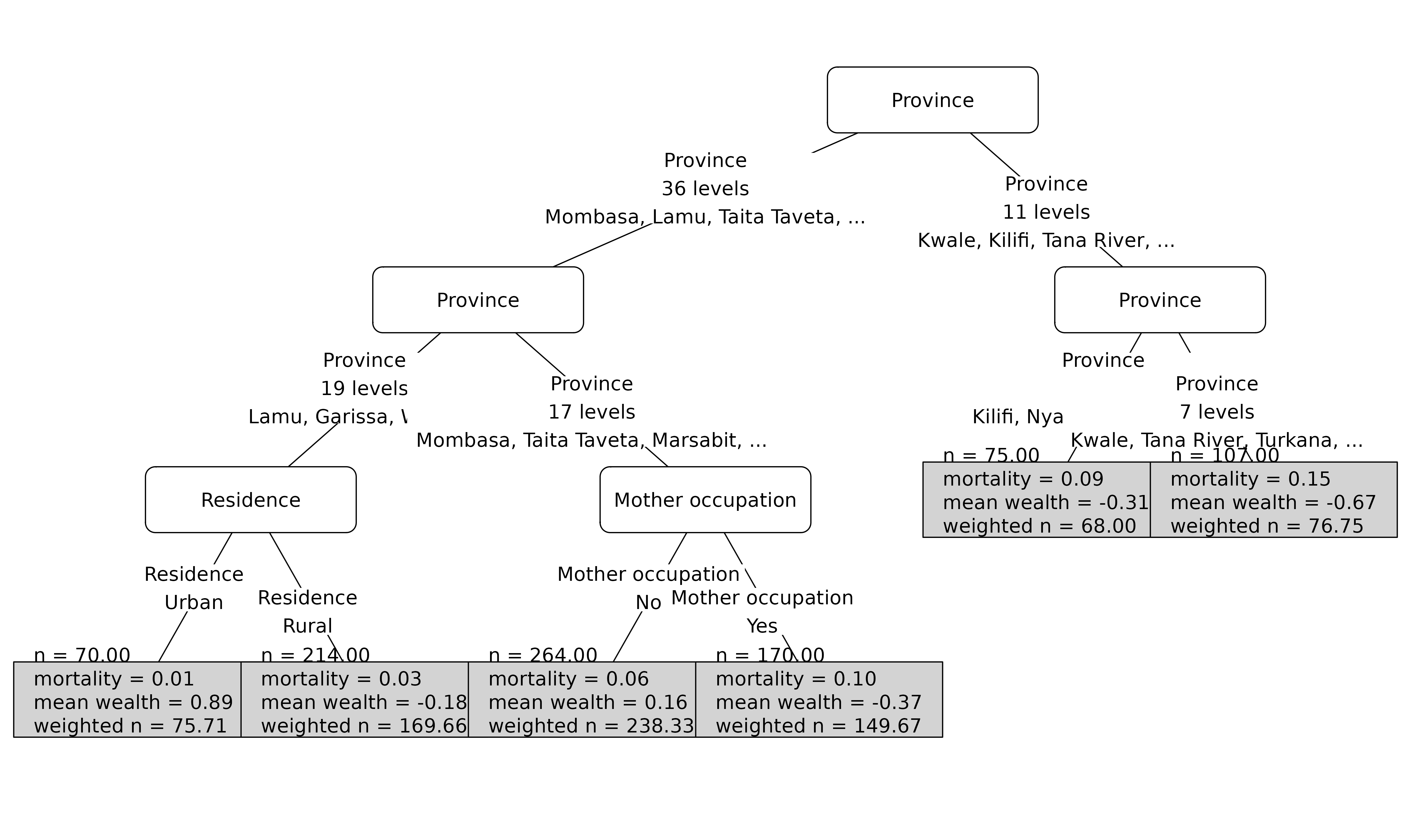
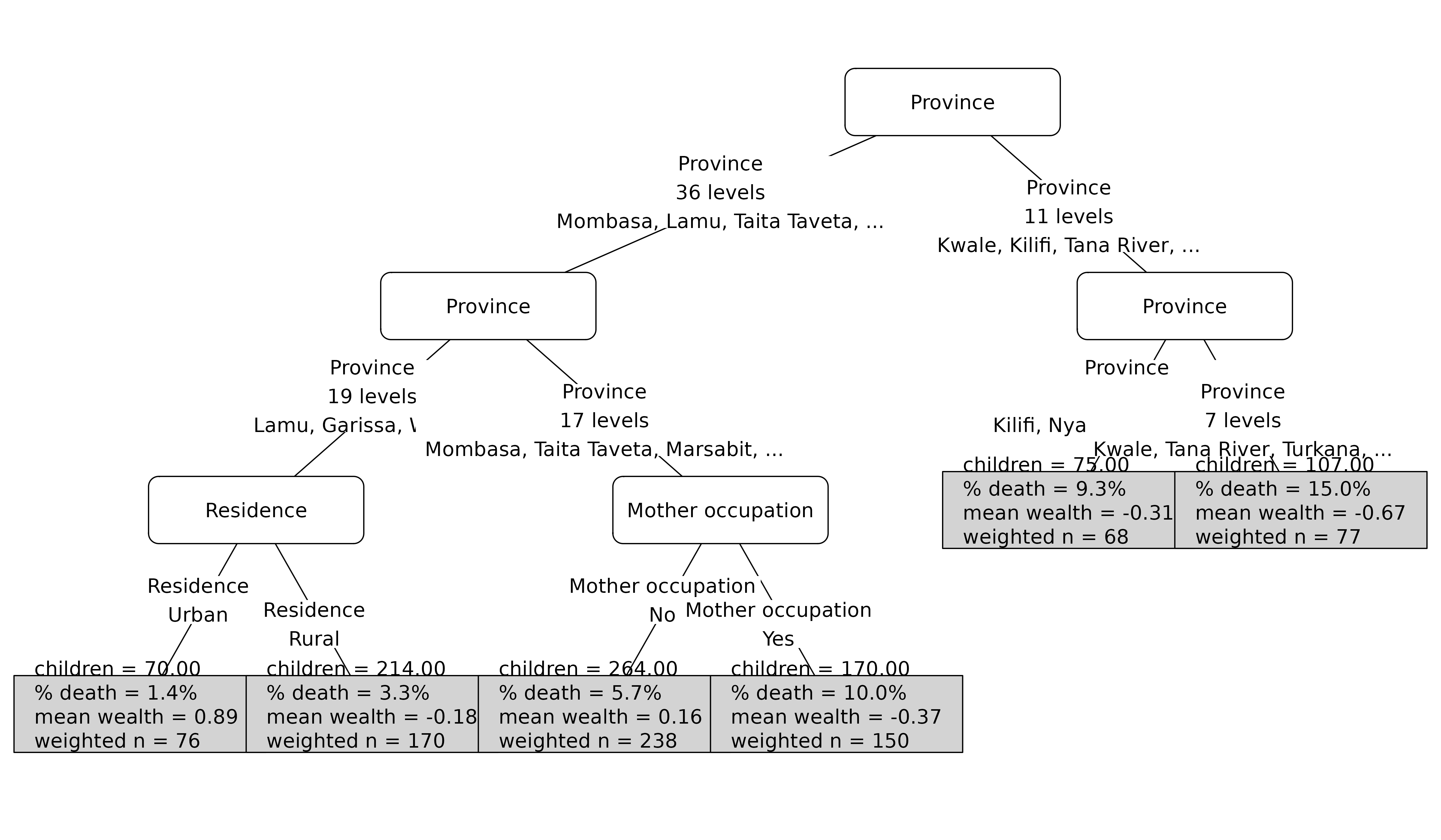
The raw output is useful, but report plots usually need shorter
labels and consistent number formatting. Use stat_labels to
rename the rows in the terminal panels and stat_formatters
to format the values.
plot(
  tree,
  data = plot_data,
  var_labels = plot_labels,
  plural_overrides = c(Province = "provinces"),
  terminal_stats = node_stats,
  stat_labels = c(
    n = "children",
    mortality = "% death",
    mean_wealth = "mean wealth",
    weighted_n = "weighted n"
  ),
  stat_formatters = list(
    mortality = function(x) sprintf("%.1f%%", 100 * x),
    mean_wealth = function(x) sprintf("%.2f", x),
    weighted_n = function(x) format(round(x), big.mark = ",")
  )
)
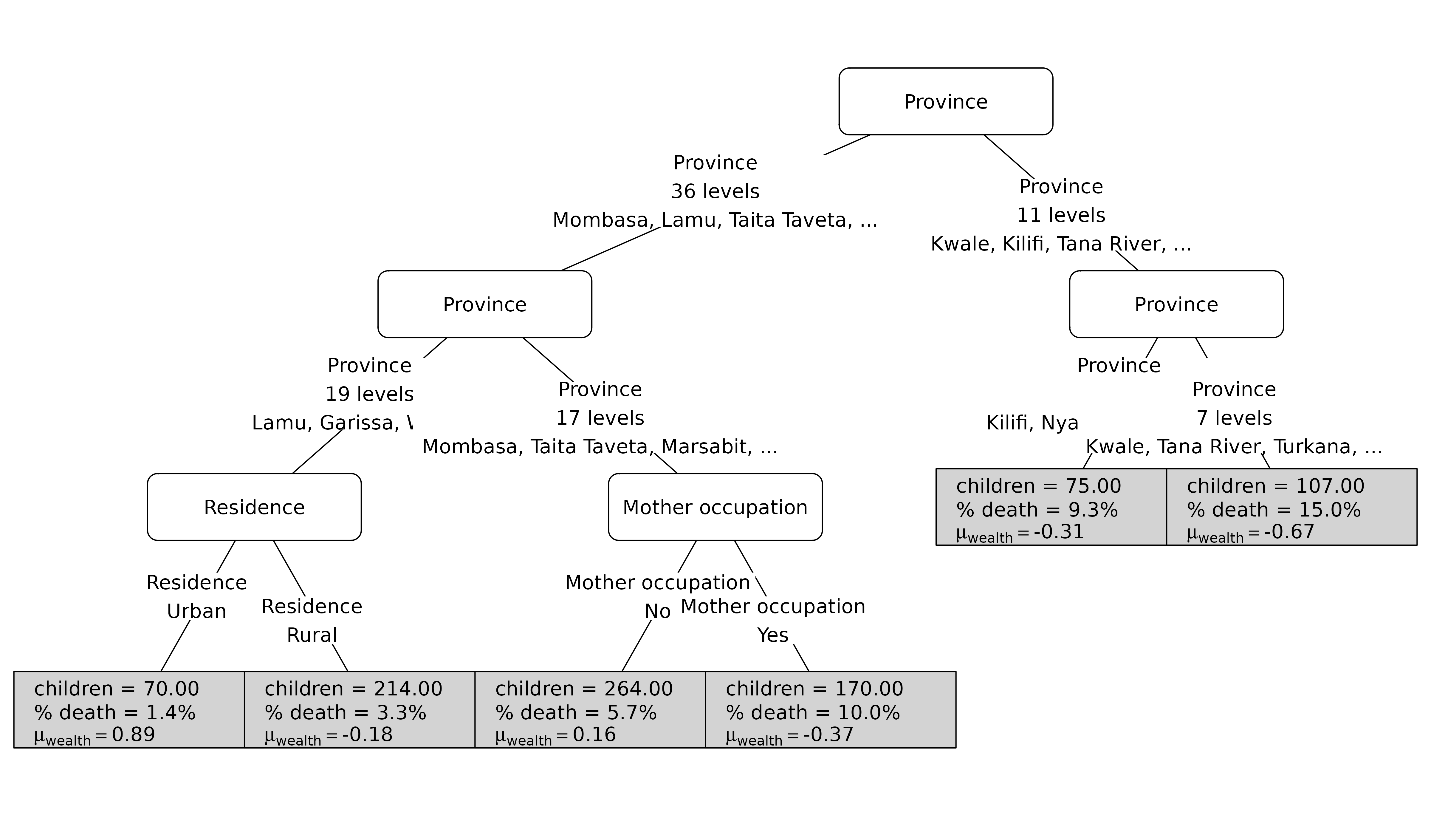
stat_labels can also contain plotmath expressions. A
named list is useful when mixing expressions and plain text labels.
plot(
  tree,
  data = plot_data,
  var_labels = plot_labels,
  plural_overrides = c(Province = "provinces"),
  terminal_stats = list(
    n = nrow,
    mortality = function(df) mean(df$deadu5_num),
    mean_wealth = function(df) mean(df$wealth)
  ),
  stat_labels = list(
    n = "children",
    mortality = "% death",
    mean_wealth = expression(mu[wealth])
  ),
  stat_formatters = list(
    mortality = function(x) sprintf("%.1f%%", 100 * x),
    mean_wealth = function(x) sprintf("%.2f", x)
  )
)
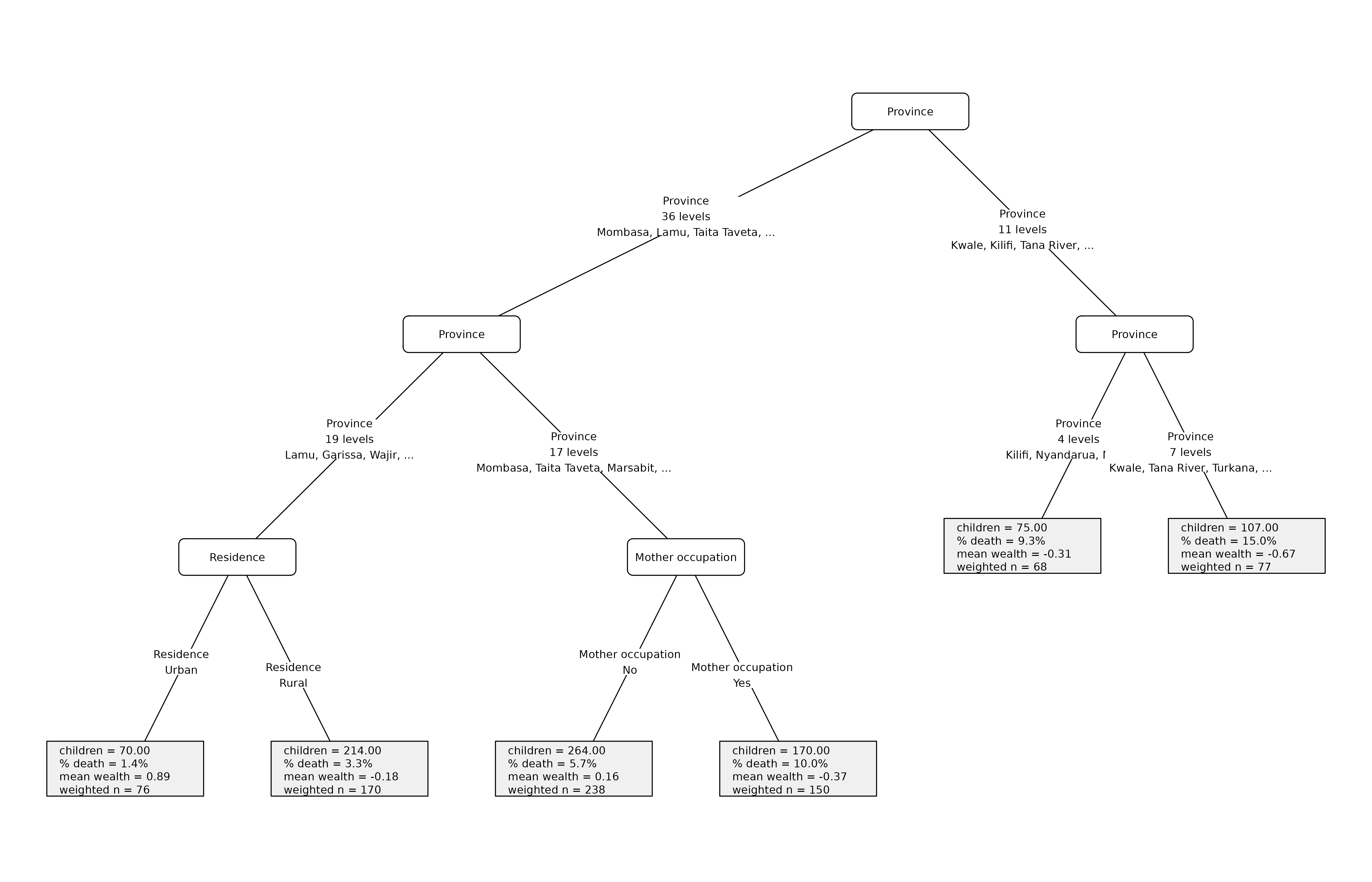
Tune Panel Size And Typography
When terminal nodes contain several statistics, increase the
terminal-panel height and width with tp_args. Font size is
controlled with gp, a standard grid::gpar()
object passed through to the underlying plot method.
plot(
  tree,
  data = plot_data,
  gp = grid::gpar(fontsize = 8),
  var_labels = plot_labels,
  plural_overrides = c(Province = "provinces"),
  terminal_stats = node_stats,
  stat_labels = c(
    n = "children",
    mortality = "% death",
    mean_wealth = "mean wealth",
    weighted_n = "weighted n"
  ),
  stat_formatters = list(
    mortality = function(x) sprintf("%.1f%%", 100 * x),
    mean_wealth = function(x) sprintf("%.2f", x),
    weighted_n = function(x) format(round(x), big.mark = ",")
  ),
  terminal_fill = "#f0f0f0",
  tp_args = list(
    width_lines = 12,
    height_lines = 4.2
  ),
  tnex = 0.9
)
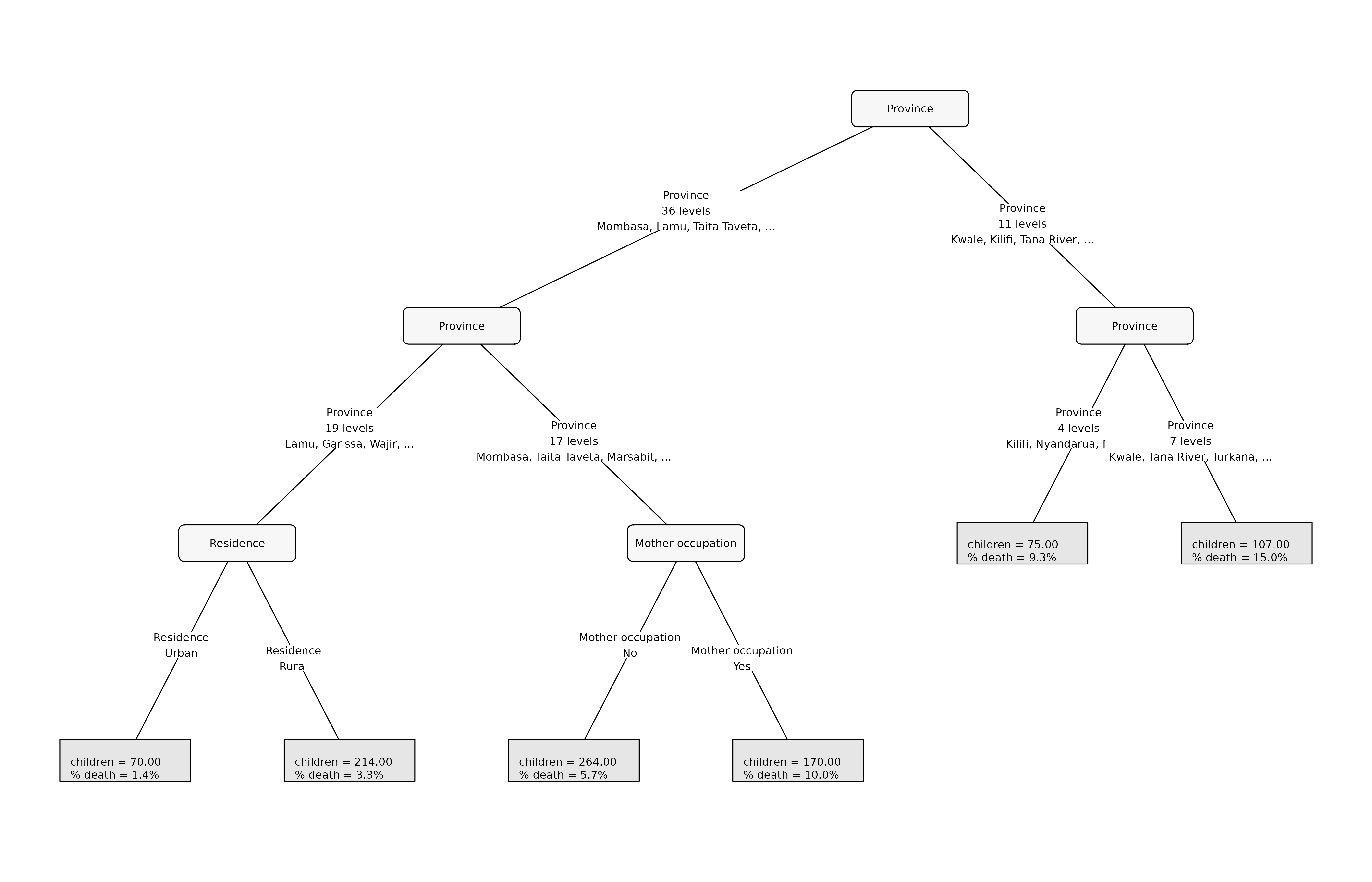
The fill colors for the three custom panels are controlled
separately: edge_fill, inner_fill, and
terminal_fill.
plot(
  tree,
  data = plot_data,
  gp = grid::gpar(fontsize = 8),
  var_labels = plot_labels,
  plural_overrides = c(Province = "provinces"),
  terminal_stats = list(
    n = nrow,
    mortality = function(df) mean(df$deadu5_num)
  ),
  stat_labels = c(
    n = "children",
    mortality = "% death"
  ),
  stat_formatters = list(
    mortality = function(x) sprintf("%.1f%%", 100 * x)
  ),
  edge_fill = "white",
  inner_fill = "#f7f7f7",
  terminal_fill = "#e6e6e6",
  tp_args = list(
    width_lines = 10,
    height_lines = 3.2
  )
)
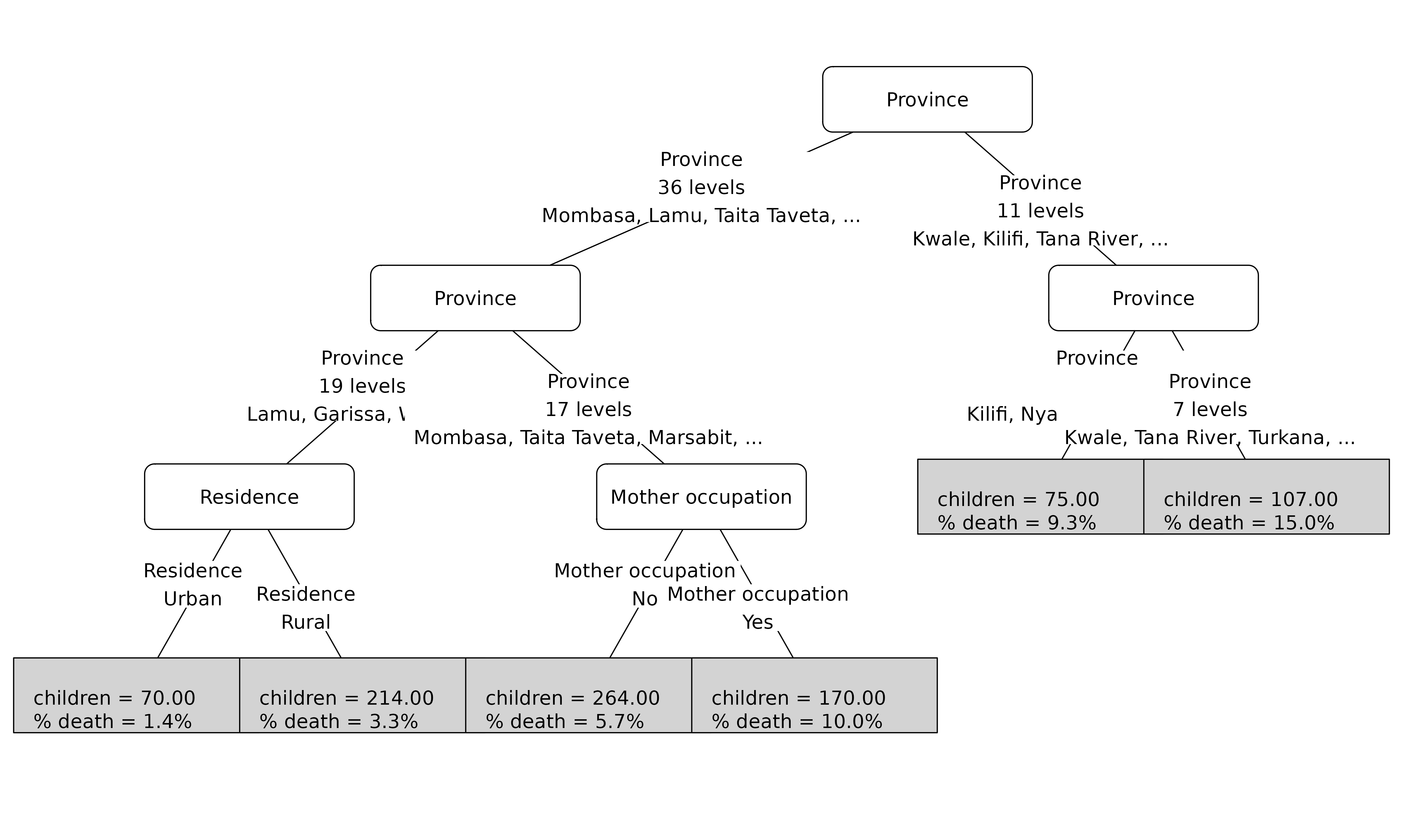
Hide Split Test P-Values
ci_tree() uses direct greedy split search, not
conditional-inference testing. The internal panel can display a p-value
when one is present on the node, but for many concentration-index tree
reports it is clearer to show only the split variable.
plot(
  tree,
  data = plot_data,
  var_labels = plot_labels,
  plural_overrides = c(Province = "provinces"),
  terminal_stats = list(
    n = nrow,
    mortality = function(df) mean(df$deadu5_num)
  ),
  stat_labels = c(
    n = "children",
    mortality = "% death"
  ),
  stat_formatters = list(
    mortality = function(x) sprintf("%.1f%%", 100 * x)
  ),
  show_p = FALSE
)
Inspect The Terminal Table Behind The Plot
Before deciding what to put in a plot, it is often helpful to inspect
the terminal-node summary table. ci_tree_terminal_summary()
returns one row per terminal node, including the subgroup rule leading
to that node.
terminal_summary <- ci_tree_terminal_summary(tree)

terminal_summary[
  order(-outcome_percent),
  .(node, n, weight, depth, ci, outcome_percent, rule)
]
#>     node     n    weight depth         ci outcome_percent
#>    <int> <int>     <num> <int>      <num>           <num>
#> 1:    11   107  76.74582     2 0.12642519      28.2512544
#> 2:    10    75  67.99996     2 0.38445924      12.8839020
#> 3:     8   170 149.67115     3 0.21954762       8.9342047
#> 4:     7   264 238.33132     3 0.13652689       4.7413463
#> 5:     5   214 169.65834     3 0.04479042       1.5984970
#> 6:     4    70  75.70745     3 0.06452379       0.4731004
#>                                                                                                                                                                                                                                                                                                                                                                                                                                                                                                                                                      rule
#>                                                                                                                                                                                                                                                                                                                                                                                                                                                                                                                                                    <char>
#> 1:                                                                                                                                                                                                                                                                                                                                                               reg in {Kwale, Kilifi, Tana River, Nyandarua, Turkana, Samburu, Trans Nzoia, Nandi, Busia, Siaya, Homa Bay} & reg in {Kwale, Tana River, Turkana, Samburu, Trans Nzoia, Busia, Homa Bay}
#> 2:                                                                                                                                                                                                                                                                                                                                                                                                 reg in {Kwale, Kilifi, Tana River, Nyandarua, Turkana, Samburu, Trans Nzoia, Nandi, Busia, Siaya, Homa Bay} & reg in {Kilifi, Nyandarua, Nandi, Siaya}
#> 3:     reg in {Mombasa, Lamu, Taita Taveta, Garissa, Wajir, Mandera, Marsabit, Isiolo, Meru, Tharaka-Nithi, Embu, Kitui, Machakos, Makueni, Nyeri, Kirinyaga, Murang'a, Kiambu, West Pokot, Uasin Gishu, Elgeyo-Marakwet, Baringo, Laikipia, Nakuru, Narok, Kajiado, Kericho, Bomet, Kakamega, Vihiga, Bungoma, Kisumu, Migori, Kisii, Nyamira, Nairobi} & reg in {Mombasa, Taita Taveta, Marsabit, Meru, Tharaka-Nithi, Kitui, Machakos, Makueni, Kiambu, Uasin Gishu, Nakuru, Kajiado, Kericho, Kakamega, Bungoma, Kisumu, Migori} & unskilled in {Yes}
#> 4:      reg in {Mombasa, Lamu, Taita Taveta, Garissa, Wajir, Mandera, Marsabit, Isiolo, Meru, Tharaka-Nithi, Embu, Kitui, Machakos, Makueni, Nyeri, Kirinyaga, Murang'a, Kiambu, West Pokot, Uasin Gishu, Elgeyo-Marakwet, Baringo, Laikipia, Nakuru, Narok, Kajiado, Kericho, Bomet, Kakamega, Vihiga, Bungoma, Kisumu, Migori, Kisii, Nyamira, Nairobi} & reg in {Mombasa, Taita Taveta, Marsabit, Meru, Tharaka-Nithi, Kitui, Machakos, Makueni, Kiambu, Uasin Gishu, Nakuru, Kajiado, Kericho, Kakamega, Bungoma, Kisumu, Migori} & unskilled in {No}
#> 5: reg in {Mombasa, Lamu, Taita Taveta, Garissa, Wajir, Mandera, Marsabit, Isiolo, Meru, Tharaka-Nithi, Embu, Kitui, Machakos, Makueni, Nyeri, Kirinyaga, Murang'a, Kiambu, West Pokot, Uasin Gishu, Elgeyo-Marakwet, Baringo, Laikipia, Nakuru, Narok, Kajiado, Kericho, Bomet, Kakamega, Vihiga, Bungoma, Kisumu, Migori, Kisii, Nyamira, Nairobi} & reg in {Lamu, Garissa, Wajir, Mandera, Isiolo, Embu, Nyeri, Kirinyaga, Murang'a, West Pokot, Elgeyo-Marakwet, Baringo, Laikipia, Narok, Bomet, Vihiga, Kisii, Nyamira, Nairobi} & rural in {Rural}
#> 6: reg in {Mombasa, Lamu, Taita Taveta, Garissa, Wajir, Mandera, Marsabit, Isiolo, Meru, Tharaka-Nithi, Embu, Kitui, Machakos, Makueni, Nyeri, Kirinyaga, Murang'a, Kiambu, West Pokot, Uasin Gishu, Elgeyo-Marakwet, Baringo, Laikipia, Nakuru, Narok, Kajiado, Kericho, Bomet, Kakamega, Vihiga, Bungoma, Kisumu, Migori, Kisii, Nyamira, Nairobi} & reg in {Lamu, Garissa, Wajir, Mandera, Isiolo, Embu, Nyeri, Kirinyaga, Murang'a, West Pokot, Elgeyo-Marakwet, Baringo, Laikipia, Narok, Bomet, Vihiga, Kisii, Nyamira, Nairobi} & rural in {Urban}
For custom plot statistics, the same node assignment logic is
available through tree_build_terminal_stats().
tree_build_terminal_stats(
  fit = tree,
  data = plot_data,
  stat_funs = node_stats
)
#>   node_id   n  mortality mean_wealth weighted_n
#> 1       4  70 0.01428571   0.8897726   75.70745
#> 2       5 214 0.03271028  -0.1843523  169.65834
#> 3       7 264 0.05681818   0.1587406  238.33132
#> 4       8 170 0.10000000  -0.3717075  149.67115
#> 5      10  75 0.09333333  -0.3076070   67.99996
#> 6      11 107 0.14953271  -0.6683169   76.74582
This is a good debugging step: if a statistic does not look right in the plot, check the table first.
Plot A Forest Surrogate
ci_forest() itself is an ensemble, so there is no single
tree structure to draw. For interpretation, fit a surrogate tree to the
forest predictions with ci_forest_surrogate() and plot the
surrogate fit.
set.seed(20260521)

forest <- ci_forest(
  formula = cbind(wealth, deadu5_num) ~ rural + ed + reg + unskilled,
  data = plot_data,
  rank_name = "wealth",
  outcome_name = "deadu5_num",
  weights = plot_data$sample_weight,
  ntree = 12L,
  mtry = 2L,
  control = ci_tree_control(
    minsplit = 120,
    minbucket = 60,
    minprob = 0.05,
    maxdepth = 3
  )
)

surrogate <- ci_forest_surrogate(
  forest,
  data = plot_data,
  formula = cbind(wealth, deadu5_num) ~ rural + ed + reg + unskilled,
  rank_name = "wealth",
  weights = plot_data$sample_weight,
  prediction_name = "forest_risk",
  control = ci_tree_control(
    minsplit = 120,
    minbucket = 60,
    minprob = 0.05,
    maxdepth = 2
  )
)
plot(
  surrogate$fit,
  data = surrogate$data,
  gp = grid::gpar(fontsize = 8),
  var_labels = plot_labels,
  plural_overrides = c(Province = "provinces"),
  terminal_stats = list(
    n = nrow,
    predicted_risk = function(df) mean(df$forest_risk),
    mean_wealth = function(df) mean(df$wealth)
  ),
  stat_labels = c(
    n = "children",
    predicted_risk = "predicted risk",
    mean_wealth = "mean wealth"
  ),
  stat_formatters = list(
    predicted_risk = function(x) sprintf("%.1f%%", 100 * x),
    mean_wealth = function(x) sprintf("%.2f", x)
  ),
  terminal_fill = "#eeeeee",
  tp_args = list(
    width_lines = 12,
    height_lines = 3.6
  )
)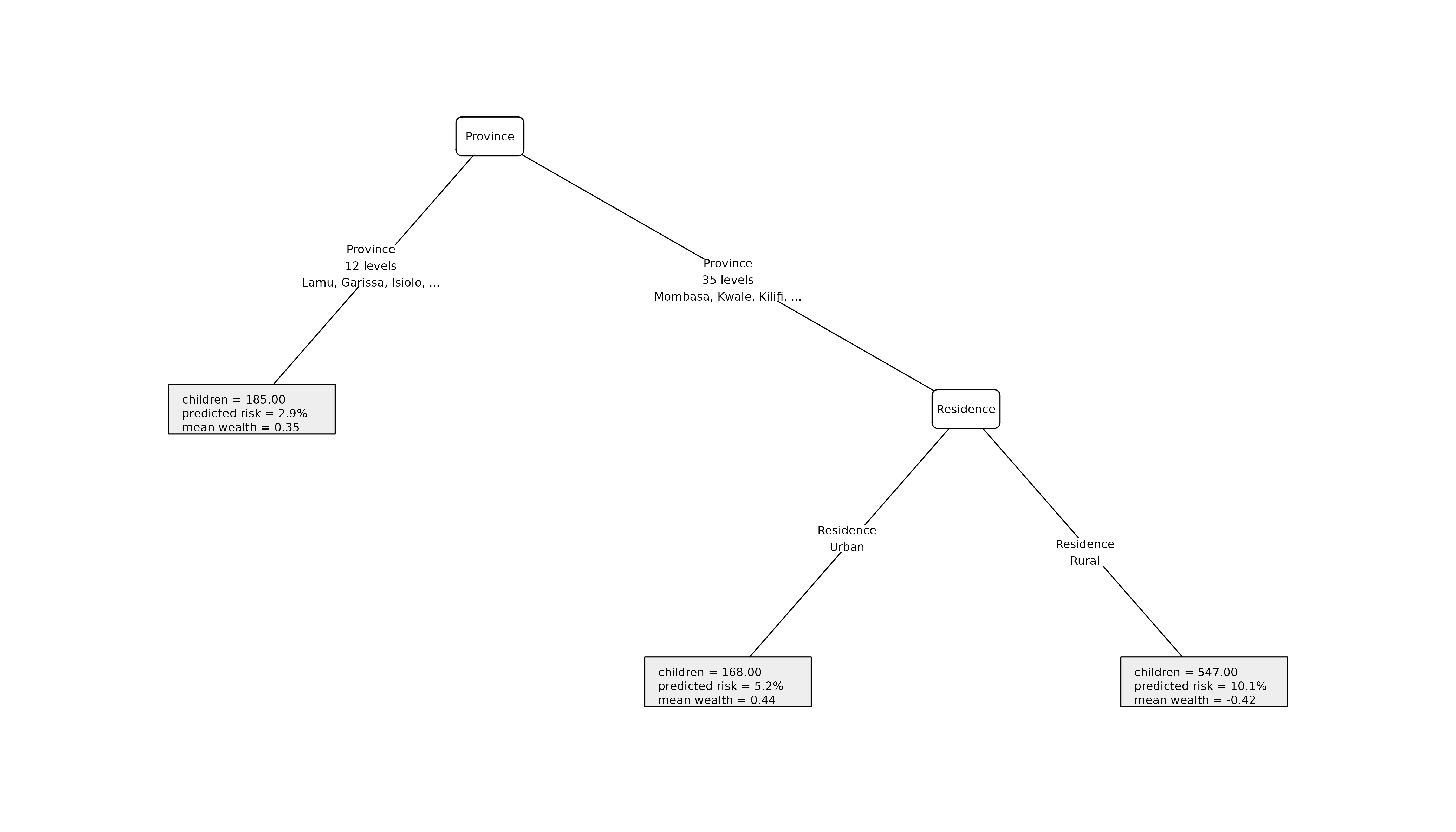
The surrogate plot should be described as an interpretation of the forest predictions, not as the forest itself.
Saving Plots
Tree plots are drawn with grid graphics. In scripts,
open a graphics device, call plot(), and then close the
device.
grDevices::png(
  filename = "ci-tree-plot.png",
  width = 2400,
  height = 1600,
  res = 200,
  bg = "white"
)

plot(
  tree,
  data = plot_data,
  gp = grid::gpar(fontsize = 8),
  var_labels = plot_labels,
  plural_overrides = c(Province = "provinces"),
  terminal_stats = node_stats,
  stat_labels = c(
    n = "children",
    mortality = "% death",
    mean_wealth = "mean wealth",
    weighted_n = "weighted n"
  ),
  stat_formatters = list(
    mortality = function(x) sprintf("%.1f%%", 100 * x),
    mean_wealth = function(x) sprintf("%.2f", x),
    weighted_n = function(x) format(round(x), big.mark = ",")
  ),
  tp_args = list(
    width_lines = 12,
    height_lines = 4.2
  )
)

grDevices::dev.off()
For pkgdown or R Markdown documents, prefer chunk options such as
fig.width, fig.height, fig.bg,
and fig.alt, as shown throughout this tutorial. An opaque
figure background keeps transparent PNGs from inheriting GitHub’s dark
mode background.
Practical Defaults
A compact reporting template is:
plot(
  tree,
  data = plot_data,
  gp = grid::gpar(fontsize = 8),
  var_labels = plot_labels,
  plural_overrides = c(Province = "provinces"),
  terminal_stats = list(
    n = nrow,
    mortality = function(df) mean(df$deadu5_num),
    mean_wealth = function(df) mean(df$wealth)
  ),
  stat_labels = c(
    n = "children",
    mortality = "% death",
    mean_wealth = "mean wealth"
  ),
  stat_formatters = list(
    mortality = function(x) sprintf("%.1f%%", 100 * x),
    mean_wealth = function(x) sprintf("%.2f", x)
  ),
  terminal_fill = "#f0f0f0",
  tp_args = list(
    width_lines = 11,
    height_lines = 3.6
  ),
  tnex = 0.9
)
The most important choices are not graphical. Choose terminal statistics that answer the analysis question, keep labels short enough to read, and state clearly whether a plotted tree is the fitted tree or a surrogate for forest predictions.