Introduction
ineqTrees is built around an applied question: how is a
health outcome distributed across a socioeconomic ranking, and which
interpretable subgroups account for the remaining inequality?
The package-native workflow in ineqTrees answers that
question directly with ci_tree(), ci_forest(),
and the package’s own tuning helpers. In some projects, however, it is
useful to fit the same models inside the tidymodels framework so they
can move through parsnip, workflows,
rsample, dials, and tune.
This article follows the same Kenya child-survival example used in the core introductory vignette. It keeps the same substantive concepts:
- the root concentration index as the baseline inequality benchmark;
- concentration-index tree criteria such as
"CI","CIg","CIc", and"L"; - interpretable tree plots and terminal-node summaries;
- forest risk estimates and model-based inequality summaries.
The difference is that the model specifications, resampling, and tuning are now handled through tidymodels.
library(ineqTrees)
library(parsnip)
library(workflows)
library(rsample)
library(dials)
#> Loading required package: scales
library(tune)
library(yardstick)
library(hardhat)
library(data.table)
#>
#> Attaching package: 'data.table'
#> The following object is masked from 'package:base':
#>
#>     %notin%

register_ineqtrees_parsnip()

data(kenya, package = "ineqTrees")
setDT(kenya)
1. Prepare the analysis table
The ingredients are the same as in the package-native workflow: a socioeconomic rank, a health outcome, interpretable predictors, and case weights.
analysis_vars <- c(
  "wealth",
  "deadu5_num",
  "rural",
  "ed",
  "reg",
  "unskilled",
  "sample_weight"
)

kenya_child <- kenya[
  complete.cases(kenya[, ..analysis_vars]),
  ..analysis_vars
]

kenya_child[
  ,
  .(
    children = .N,
    mortality = mean(deadu5_num),
    mean_wealth = mean(wealth)
  ),
  by = rural
]
#>     rural children  mortality mean_wealth
#>    <fctr>    <int>      <num>       <num>
#> 1:  Rural    15277 0.08496433  -0.3046825
#> 2:  Urban     4766 0.03755770   0.5498055
For a fast article build we use a reproducible subset. The analysis object is stored as a regular data frame because that is the most natural input type for tidymodels workflows.
set.seed(20260516)

kenya_model <- as.data.frame(
  kenya_child[sample.int(.N, min(800L, .N))]
)

kenya_model$case_wt <- hardhat::importance_weights(kenya_model$sample_weight)

predictors <- c("rural", "ed", "reg", "unskilled")
criterion_types <- c("CI", "CIg", "CIc", "L")
predictor_formula <- deadu5_num ~ wealth + rural + ed + reg + unskilled

plot_labels <- c(
  rural = "Residence",
  ed = "Mother education",
  reg = "Province",
  unskilled = "Mother occupation"
)

head(kenya_model[, c("wealth", "deadu5_num", "rural", "ed", "case_wt")])
#>       wealth deadu5_num rural             ed   case_wt
#> 1 -1.0920512          0 Rural    a education 0.4085297
#> 2 -0.9328643          0 Rural b no education 0.5599644
#> 3 -1.4867217          0 Rural b no education 0.2135889
#> 4 -0.5767841          0 Rural    a education 0.4242640
#> 5 -1.4060327          0 Rural b no education 0.3385087
#> 6 -1.1988336          0 Rural    a education 0.8798417
The formula is written in the tidymodels style, with
deadu5_num as the outcome and wealth on the
right-hand side. The ineqTrees parsnip bridge uses
wealth as rank_name, rebuilds the two-column
concentration-index response internally, and removes wealth
from the split-search predictors.
2. Measure socioeconomic inequality at the root
The root concentration index is still the benchmark before any subgrouping. It gives the level of whole-sample inequality that the tree or forest will try to explain.
root_response <- cbind(
  rank = kenya_model$wealth,
  outcome = kenya_model$deadu5_num
)

root_weights <- kenya_model$sample_weight

whole_sample_ci <- data.table(criterion = criterion_types)[
  ,
  .(
    root_ci_index = ci_factory(criterion)(root_response, root_weights)
  ),
  by = criterion
]
#> Warning: `type = "L"` uses observed socioeconomic levels rather than fractional
#> ranks. The first response column contains negative values; the
#> Erreygers-Kessels level-dependent index is intended for meaningful ratio-scale
#> socioeconomic levels such as income, consumption, or expenditure. Centered
#> wealth-index scores with negative values may be inappropriate for this
#> criterion. See https://doi.org/10.3390/ijerph14070673. This warning is shown
#> once per R session.

whole_sample_ci
#>    criterion root_ci_index
#>       <char>         <num>
#> 1:        CI    0.25733964
#> 2:       CIg    0.01731193
#> 3:       CIc    0.06924773
#> 4:         L    0.43410142
Each concentration-index criterion has its own scale, so fitted
models should always be compared with the root benchmark for the same
type.
3. Fit trees with different concentration indices through tidymodels
The first question is the same one asked in the package-native vignette: what happens if the tree is fitted under different concentration-index objectives?
Here the model specification is created with
decision_tree() and
set_engine("ineqTrees", ...), but the underlying fitted
object is still a ci_tree. That means the same validation
and plotting methods remain available after fitting.
fit_tree_with_type <- function(ci_type) {
  spec <- decision_tree(
    tree_depth = 3L,
    min_n = 60L
  ) |>
    set_engine(
      "ineqTrees",
      rank_name = "wealth",
      outcome_name = "deadu5_num",
      type = ci_type,
      minsplit = 120L,
      minprob = 0.05,
      min_gain = 0,
      min_relative_gain = 0
    ) |>
    set_mode("regression")

  fit(
    spec,
    predictor_formula,
    data = kenya_model,
    case_weights = kenya_model$case_wt
  )
}

tree_by_type <- setNames(
  lapply(criterion_types, fit_tree_with_type),
  criterion_types
)

type_comparison <- rbindlist(lapply(names(tree_by_type), function(ci_type) {
  fit_object <- tree_by_type[[ci_type]]$fit

  data.table(
    type = ci_type,
    terminal_nodes = length(partykit::nodeids(fit_object, terminal = TRUE)),
    validation_gain = ci_tree_validation_gain(
      fit = fit_object,
      new_data = kenya_model,
      rank_name = "wealth",
      outcome_name = "deadu5_num",
      weights = kenya_model$sample_weight,
      type = ci_type
    )
  )
}))

type_comparison[order(-validation_gain)]
#>      type terminal_nodes validation_gain
#>    <char>          <int>           <num>
#> 1:      L              4     0.378268187
#> 2:     CI              6     0.191485406
#> 3:    CIc              4     0.030791748
#> 4:    CIg              4     0.007697937
This comparison is still on the inequality scale: larger validation gain means the terminal-node partition removes more concentration-index impurity than the unsplit root. In the next section we work with a single interpretable tree so the mechanics of the tidymodels fit are easy to see.
4. Fit a single inequality-aware tree
decision_tree() supplies the generic tree controls. The
engine-specific arguments describe the inequality problem itself: which
column is the rank, which column is the outcome, and which
concentration-index criterion should be optimized.
tree_spec <- decision_tree(
  tree_depth = 3L,
  min_n = 60L
) |>
  set_engine(
    "ineqTrees",
    rank_name = "wealth",
    outcome_name = "deadu5_num",
    type = "CI",
    minsplit = 120L,
    minprob = 0.05,
    min_gain = 0,
    min_relative_gain = 0
  ) |>
  set_mode("regression")

tree_spec
#> Decision Tree Model Specification (regression)
#>
#> Main Arguments:
#>   tree_depth = 3
#>   min_n = 60
#>
#> Engine-Specific Arguments:
#>   rank_name = wealth
#>   outcome_name = deadu5_num
#>   type = CI
#>   minsplit = 120
#>   minprob = 0.05
#>   min_gain = 0
#>   min_relative_gain = 0
#>
#> Computational engine: ineqTrees
tree_fit <- fit(
  tree_spec,
  predictor_formula,
  data = kenya_model,
  case_weights = kenya_model$case_wt
)

tree_fit$fit
Greedy concentration-index tree
Formula:
cbind(wealth, deadu5_num) ~ rural + ed + reg + unskilled
Criterion: CI Tree size: 5 inner
nodes, 6 terminal nodes, max depth 3
| node | n | weight | depth | CI | outcome_mean | outcome_percent | rule |
|---|---|---|---|---|---|---|---|
| 11 | 246 | 201.20653 | 2 | 0.185 | 0.207 | 20.7 | reg in {Kwale, Kilifi, Tana River, Garissa, Wajir, Mandera, Embu, Machakos, Makueni, Nyeri, Murang’a, Turkana, Uasin Gishu, Baringo, Nakuru, Narok, Kajiado, Bomet, Kakamega, Siaya, Kisumu, Homa Bay, Kisii} & reg in {Kilifi, Tana River, Wajir, Mandera, Embu, Machakos, Makueni, Nyeri, Baringo, Narok, Kakamega, Siaya, Kisumu, Homa Bay} |
| 10 | 73 | 89.72991 | 3 | 0.065 | 0.051 | 5.1 | reg in {Kwale, Kilifi, Tana River, Garissa, Wajir, Mandera, Embu, Machakos, Makueni, Nyeri, Murang’a, Turkana, Uasin Gishu, Baringo, Nakuru, Narok, Kajiado, Bomet, Kakamega, Siaya, Kisumu, Homa Bay, Kisii} & reg in {Kwale, Garissa, Murang’a, Turkana, Uasin Gishu, Nakuru, Kajiado, Bomet, Kisii} & unskilled in {Yes} |
| 9 | 126 | 107.85862 | 3 | 0.029 | 0.021 | 2.1 | reg in {Kwale, Kilifi, Tana River, Garissa, Wajir, Mandera, Embu, Machakos, Makueni, Nyeri, Murang’a, Turkana, Uasin Gishu, Baringo, Nakuru, Narok, Kajiado, Bomet, Kakamega, Siaya, Kisumu, Homa Bay, Kisii} & reg in {Kwale, Garissa, Murang’a, Turkana, Uasin Gishu, Nakuru, Kajiado, Bomet, Kisii} & unskilled in {No} |
| 6 | 99 | 85.82087 | 3 | 0.018 | 0.004 | 0.4 | reg in {Mombasa, Lamu, Taita Taveta, Marsabit, Isiolo, Meru, Tharaka-Nithi, Kitui, Nyandarua, Kirinyaga, Kiambu, West Pokot, Samburu, Trans Nzoia, Elgeyo-Marakwet, Nandi, Laikipia, Kericho, Vihiga, Bungoma, Busia, Migori, Nyamira, Nairobi} & rural in {Rural} & unskilled in {Yes} |
| 5 | 165 | 149.19428 | 3 | 0.000 | 0.000 | 0.0 | reg in {Mombasa, Lamu, Taita Taveta, Marsabit, Isiolo, Meru, Tharaka-Nithi, Kitui, Nyandarua, Kirinyaga, Kiambu, West Pokot, Samburu, Trans Nzoia, Elgeyo-Marakwet, Nandi, Laikipia, Kericho, Vihiga, Bungoma, Busia, Migori, Nyamira, Nairobi} & rural in {Rural} & unskilled in {No} |
| 3 | 91 | 91.85254 | 2 | 0.000 | 0.000 | 0.0 | reg in {Mombasa, Lamu, Taita Taveta, Marsabit, Isiolo, Meru, Tharaka-Nithi, Kitui, Nyandarua, Kirinyaga, Kiambu, West Pokot, Samburu, Trans Nzoia, Elgeyo-Marakwet, Nandi, Laikipia, Kericho, Vihiga, Bungoma, Busia, Migori, Nyamira, Nairobi} & rural in {Urban} |
The fitted object inside the parsnip model fit is a
ci_tree, so the usual terminal-node summary remains
available.
terminal_summary <- ci_tree_terminal_summary(tree_fit$fit)

terminal_summary[
  order(-outcome_percent),
  .(node, n, depth, ci, outcome_percent, rule)
]
#>     node     n depth         ci outcome_percent
#>    <int> <int> <int>      <num>           <num>
#> 1:    11   246     2 0.18490378      20.6916015
#> 2:    10    73     3 0.06508276       5.1195621
#> 3:     9   126     3 0.02929641       2.0668519
#> 4:     6    99     3 0.01846145       0.4210864
#> 5:     3    91     2 0.00000000       0.0000000
#> 6:     5   165     3 0.00000000       0.0000000
#>                                                                                                                                                                                                                                                                                                                                              rule
#>                                                                                                                                                                                                                                                                                                                                            <char>
#> 1: reg in {Kwale, Kilifi, Tana River, Garissa, Wajir, Mandera, Embu, Machakos, Makueni, Nyeri, Murang'a, Turkana, Uasin Gishu, Baringo, Nakuru, Narok, Kajiado, Bomet, Kakamega, Siaya, Kisumu, Homa Bay, Kisii} & reg in {Kilifi, Tana River, Wajir, Mandera, Embu, Machakos, Makueni, Nyeri, Baringo, Narok, Kakamega, Siaya, Kisumu, Homa Bay}
#> 2:                    reg in {Kwale, Kilifi, Tana River, Garissa, Wajir, Mandera, Embu, Machakos, Makueni, Nyeri, Murang'a, Turkana, Uasin Gishu, Baringo, Nakuru, Narok, Kajiado, Bomet, Kakamega, Siaya, Kisumu, Homa Bay, Kisii} & reg in {Kwale, Garissa, Murang'a, Turkana, Uasin Gishu, Nakuru, Kajiado, Bomet, Kisii} & unskilled in {Yes}
#> 3:                     reg in {Kwale, Kilifi, Tana River, Garissa, Wajir, Mandera, Embu, Machakos, Makueni, Nyeri, Murang'a, Turkana, Uasin Gishu, Baringo, Nakuru, Narok, Kajiado, Bomet, Kakamega, Siaya, Kisumu, Homa Bay, Kisii} & reg in {Kwale, Garissa, Murang'a, Turkana, Uasin Gishu, Nakuru, Kajiado, Bomet, Kisii} & unskilled in {No}
#> 4:                                                        reg in {Mombasa, Lamu, Taita Taveta, Marsabit, Isiolo, Meru, Tharaka-Nithi, Kitui, Nyandarua, Kirinyaga, Kiambu, West Pokot, Samburu, Trans Nzoia, Elgeyo-Marakwet, Nandi, Laikipia, Kericho, Vihiga, Bungoma, Busia, Migori, Nyamira, Nairobi} & rural in {Rural} & unskilled in {Yes}
#> 5:                                                                             reg in {Mombasa, Lamu, Taita Taveta, Marsabit, Isiolo, Meru, Tharaka-Nithi, Kitui, Nyandarua, Kirinyaga, Kiambu, West Pokot, Samburu, Trans Nzoia, Elgeyo-Marakwet, Nandi, Laikipia, Kericho, Vihiga, Bungoma, Busia, Migori, Nyamira, Nairobi} & rural in {Urban}
#> 6:                                                         reg in {Mombasa, Lamu, Taita Taveta, Marsabit, Isiolo, Meru, Tharaka-Nithi, Kitui, Nyandarua, Kirinyaga, Kiambu, West Pokot, Samburu, Trans Nzoia, Elgeyo-Marakwet, Nandi, Laikipia, Kericho, Vihiga, Bungoma, Busia, Migori, Nyamira, Nairobi} & rural in {Rural} & unskilled in {No}
5. Plot the fitted tree
Because the underlying engine fit is still a ci_tree,
the same plot method works after a tidymodels fit.
The plain call is useful when you want a quick look at the tree structure.
plot(tree_fit$fit)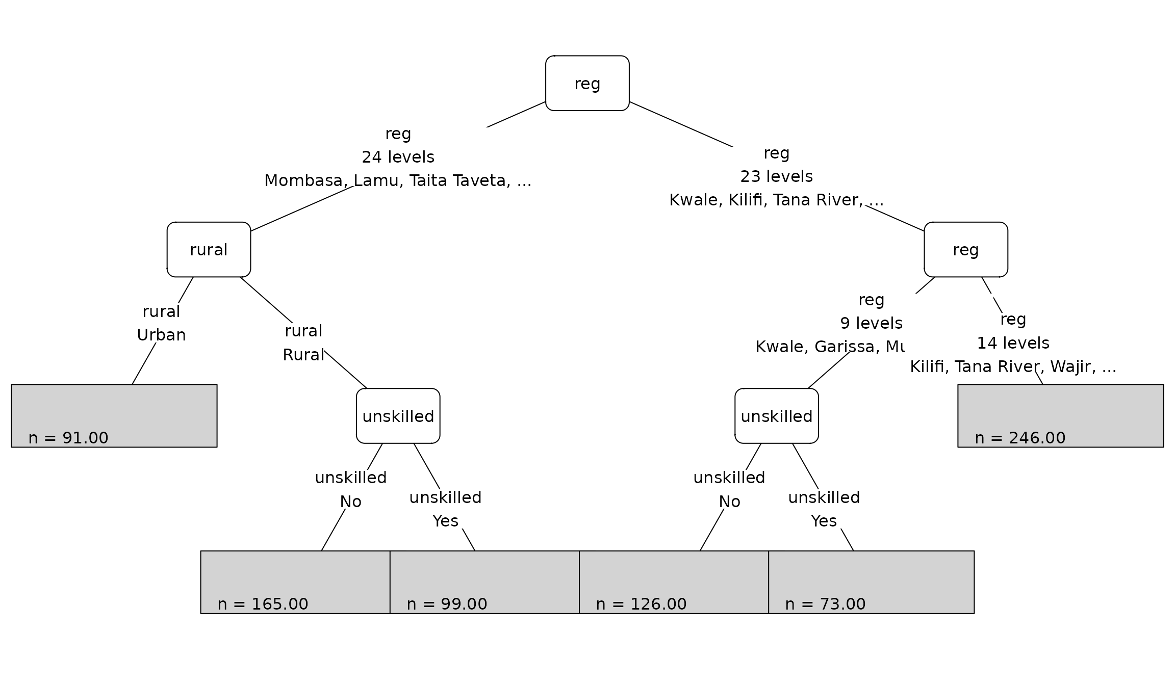
For reporting, the more useful plot is the enriched version with readable labels and terminal-node summaries.
plot(
  tree_fit$fit,
  data = kenya_model,
  var_labels = plot_labels,
  plural_overrides = c(Province = "provinces"),
  terminal_stats = list(
    n = nrow,
    mortality = function(df) mean(df$deadu5_num),
    mean_wealth = function(df) mean(df$wealth)
  ),
  stat_labels = c(
    n = "n",
    mortality = "% death",
    mean_wealth = "mean wealth"
  ),
  stat_formatters = list(
    mortality = function(x) sprintf("%.1f%%", 100 * x),
    mean_wealth = function(x) sprintf("%.2f", x)
  )
)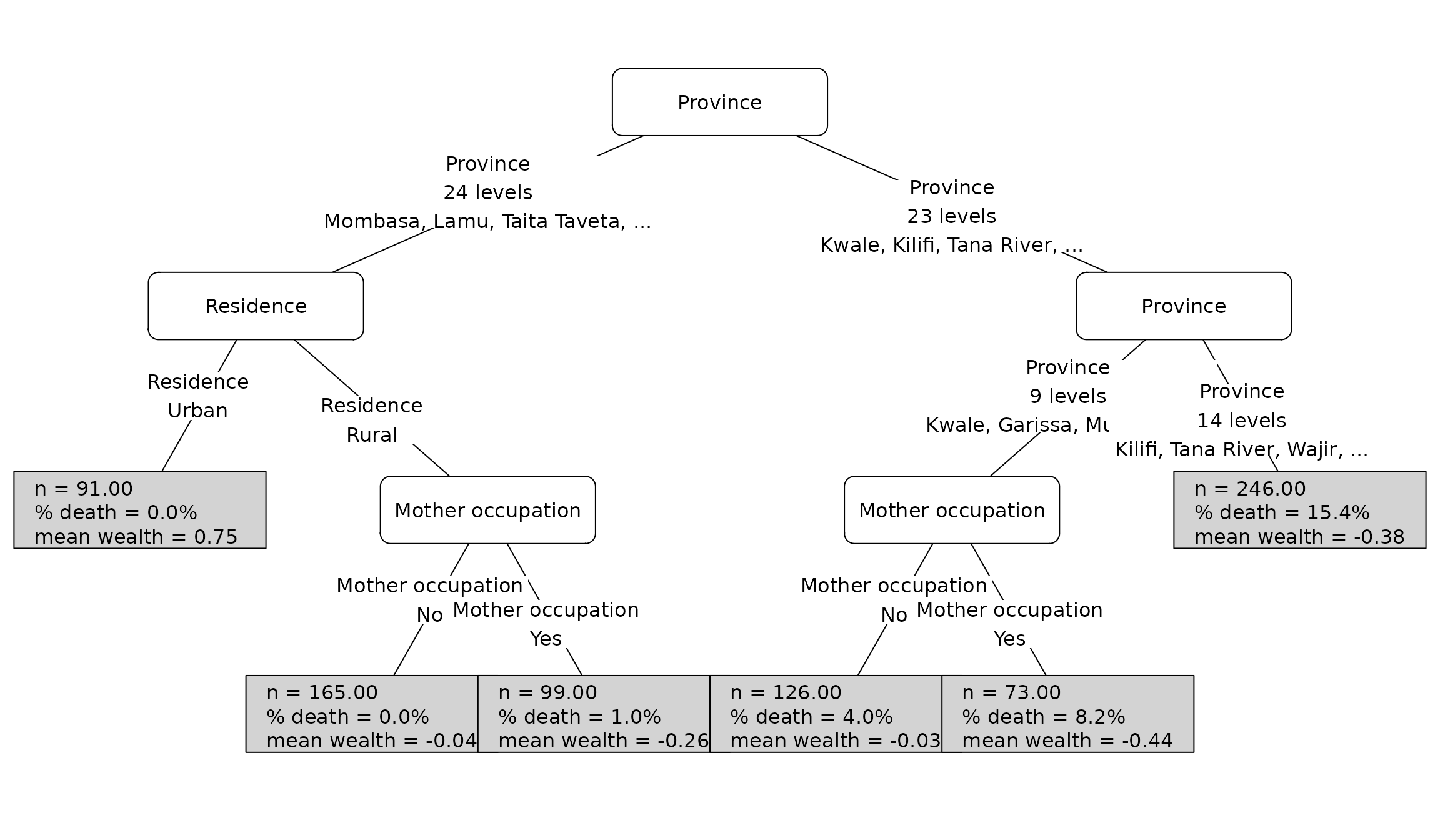
The important point is that tidymodels does not take away the
interpretability machinery already built into ineqTrees; it
just changes how the model is specified and managed.
6. Use the fitted tree as a prediction rule
The tidymodels fit returns the same kinds of predictions you would
expect from other parsnip regression models. Numeric predictions come
back as .pred, and the raw tree partition can be recovered
from the same fitted object.
tree_pred <- predict(tree_fit, new_data = kenya_model)
tree_nodes <- as.integer(
  predict(tree_fit, new_data = kenya_model, type = "raw")
)

data.table::as.data.table(kenya_model)[
  ,
  .(
    observed_mortality = mean(deadu5_num),
    mean_tree_risk = mean(tree_pred$.pred)
  )
]
#>    observed_mortality mean_tree_risk
#>                 <num>          <num>
#> 1:             0.0625     0.07207466
That raw node partition is what lets us reconnect the tidymodels fit
to the inequality interpretation. ci_gain() computes the
concentration-index gain of the fitted partition.
tree_scores <- data.frame(
  truth = kenya_model$deadu5_num,
  pred = tree_pred$.pred,
  rank = kenya_model$wealth,
  node = tree_nodes,
  weight = kenya_model$sample_weight
)

ci_gain(
  tree_scores,
  truth = truth,
  estimate = pred,
  rank = rank,
  node = node,
  case_weights = weight,
  type = "CI"
)
#> # A tibble: 1 × 3
#>   .metric .estimator .estimate
#>   <chr>   <chr>          <dbl>
#> 1 ci_gain standard       0.191
7. Tune an inequality-aware tree with tidymodels
In the package-native workflow, tune_ci_tree() handles
concentration-index tree tuning directly. In tidymodels, the equivalent
pieces are a tunable specification, a workflow, a resampling object, and
a tuning grid.
The resampling design is the same idea as before: keep the outcome reasonably balanced across folds and score candidate models on held-out data.
set.seed(20260516)

tree_folds <- vfold_cv(
  kenya_model,
  v = 3L,
  strata = deadu5_num
)

tree_folds
#> #  3-fold cross-validation using stratification
#> # A tibble: 3 × 2
#>   splits            id
#>   <list>            <chr>
#> 1 <split [533/267]> Fold1
#> 2 <split [533/267]> Fold2
#> 3 <split [534/266]> Fold3
tree_tune_spec <- decision_tree(
  tree_depth = tune(),
  min_n = tune()
) |>
  set_engine(
    "ineqTrees",
    rank_name = "wealth",
    outcome_name = "deadu5_num",
    type = "CI",
    minsplit = 120L,
    minprob = 0.05,
    min_gain = 0,
    min_relative_gain = tune()
  ) |>
  set_mode("regression")

tree_wf <- workflow() |>
  add_model(tree_tune_spec) |>
  add_formula(predictor_formula) |>
  add_case_weights(case_wt)

tree_grid <- expand.grid(
  tree_depth = c(2L, 4L),
  min_n = c(40L, 90L),
  min_relative_gain = c(0, 0.05),
  KEEP.OUT.ATTRS = FALSE,
  stringsAsFactors = FALSE
)

tree_grid
#>   tree_depth min_n min_relative_gain
#> 1          2    40              0.00
#> 2          4    40              0.00
#> 3          2    90              0.00
#> 4          4    90              0.00
#> 5          2    40              0.05
#> 6          4    40              0.05
#> 7          2    90              0.05
#> 8          4    90              0.05
To tune directly on the inequality objective, we use
ci_tuning_metric_set(). The helper uses the
.row column from tune_grid() to recover
assessment ranks and sampling weights. Numeric engine predictions retain
actual terminal-node assignments: separate leaves with equal risks
remain separate, and forest gain averages member-tree partition gains.
Training diagnostics come from each fitted analysis fold, independently
of assessment outcomes.
ci_tuning_metrics <- ci_tuning_metric_set(
  kenya_model,
  rank_name = "wealth",
  case_weight_name = "sample_weight",
  type = "CI",
  metrics = c(
    "validation_gain", "relative_validation_gain",
    "training_gain", "relative_training_gain"
  )
)
The tuning loop can still collect familiar prediction metrics
separately, but model selection is now driven by held-out
concentration-index gain. Training gain describes fit on the analysis
fold. Compare it with validation gain to assess the training-validation
gap; select parameters using the validation metric. Relative gains use
their respective fold’s root impurity and are NA when that
root is numerically zero.
set.seed(20260516)

tree_tuned <- tune_grid(
  tree_wf,
  resamples = tree_folds,
  grid = tree_grid,
  metrics = ci_tuning_metrics,
  control = control_grid(save_pred = TRUE)
)

collect_metrics(tree_tuned)
#> # A tibble: 32 × 9
#>    tree_depth min_n min_relative_gain .metric   .estimator    mean     n std_err
#>         <int> <int>             <dbl> <chr>     <chr>        <dbl> <int>   <dbl>
#>  1          2    40              0    relative… standard    0.780      3  0.0836
#>  2          2    40              0    relative… standard   -0.633      3  0.451
#>  3          2    40              0    training… standard    0.190      3  0.0349
#>  4          2    40              0    validati… standard   -0.0527     3  0.0754
#>  5          2    40              0.05 relative… standard    0.780      3  0.0836
#>  6          2    40              0.05 relative… standard   -0.631      3  0.452
#>  7          2    40              0.05 training… standard    0.190      3  0.0349
#>  8          2    40              0.05 validati… standard   -0.0517     3  0.0763
#>  9          2    90              0    relative… standard    0.733      3  0.0899
#> 10          2    90              0    relative… standard   -0.520      3  0.451
#> # ℹ 22 more rows
#> # ℹ 1 more variable: .config <chr>
show_best(tree_tuned, metric = "relative_validation_gain", n = 4)
#> # A tibble: 4 × 9
#>   tree_depth min_n min_relative_gain .metric     .estimator   mean     n std_err
#>        <int> <int>             <dbl> <chr>       <chr>       <dbl> <int>   <dbl>
#> 1          4    40              0.05 relative_v… standard   -0.427     3   0.322
#> 2          4    40              0    relative_v… standard   -0.429     3   0.321
#> 3          2    90              0    relative_v… standard   -0.520     3   0.451
#> 4          2    90              0.05 relative_v… standard   -0.520     3   0.451
#> # ℹ 1 more variable: .config <chr>

best_tree <- select_best(tree_tuned, metric = "relative_validation_gain")
best_tree
#> # A tibble: 1 × 4
#>   tree_depth min_n min_relative_gain .config
#>        <int> <int>             <dbl> <chr>
#> 1          4    40              0.05 pre0_mod6_post0
After choosing the best settings, the workflow is finalized and
refitted on the full analysis table. The final workflow still contains a
ci_tree engine fit, so the fitted partition can again be
scored with ci_gain().
final_tree_wf <- finalize_workflow(tree_wf, best_tree)
final_tree_fit <- fit(final_tree_wf, data = kenya_model)
final_tree_parsnip <- extract_fit_parsnip(final_tree_fit)

final_tree_scores <- data.frame(
  truth = kenya_model$deadu5_num,
  pred = predict(final_tree_fit, new_data = kenya_model)$.pred,
  rank = kenya_model$wealth,
  node = as.integer(
    predict(final_tree_parsnip, new_data = kenya_model, type = "raw")
  ),
  weight = kenya_model$sample_weight
)

ci_gain(
  final_tree_scores,
  truth = truth,
  estimate = pred,
  rank = rank,
  node = node,
  case_weights = weight,
  type = "CI"
)
#> # A tibble: 1 × 3
#>   .metric .estimator .estimate
#>   <chr>   <chr>          <dbl>
#> 1 ci_gain standard       0.203
8. Fit and visualize an inequality-aware forest
The forest is fitted through the same bridge, but now the generic
tidymodels arguments are trees, mtry, and
min_n.
forest_spec <- rand_forest(
  trees = 20L,
  mtry = 2L,
  min_n = 60L
) |>
  set_engine(
    "ineqTrees",
    rank_name = "wealth",
    outcome_name = "deadu5_num",
    type = "CI",
    minsplit = 120L,
    minprob = 0.05,
    maxdepth = 3L,
    min_relative_gain = 0,
    perturb = list(replace = FALSE, fraction = 0.632)
  ) |>
  set_mode("regression")

forest_spec
#> Random Forest Model Specification (regression)
#>
#> Main Arguments:
#>   mtry = 2
#>   trees = 20
#>   min_n = 60
#>
#> Engine-Specific Arguments:
#>   rank_name = wealth
#>   outcome_name = deadu5_num
#>   type = CI
#>   minsplit = 120
#>   minprob = 0.05
#>   maxdepth = 3
#>   min_relative_gain = 0
#>   perturb = list(replace = FALSE, fraction = 0.632)
#>
#> Computational engine: ineqTrees
set.seed(20260516)

forest_fit <- fit(
  forest_spec,
  predictor_formula,
  data = kenya_model,
  case_weights = kenya_model$case_wt
)

ci_forest_summary(forest_fit$fit)
#>    ntree  mtry   type     n mean_outcome mean_prediction outcome_ci
#>    <int> <int> <char> <int>        <num>           <num>      <num>
#> 1:    20     2     CI   800    0.0672727      0.06566328  0.2573396
#>    prediction_ci mean_terminal_nodes mean_max_depth
#>            <num>               <num>          <num>
#> 1:    0.04956804                2.45           1.35
The forest produces fitted risks. Because an ensemble has no single
terminal node assignment, we first keep the fitted risk table and then
score a compact surrogate tree with ci_gain().
forest_pred <- predict(forest_fit, new_data = kenya_model)

forest_scores <- data.frame(
  truth = kenya_model$deadu5_num,
  pred = forest_pred$.pred,
  rank = kenya_model$wealth,
  weight = kenya_model$sample_weight
)

head(forest_scores)
#>   truth       pred       rank    weight
#> 1     0 0.09710381 -1.0920512 0.4085297
#> 2     0 0.02940914 -0.9328643 0.5599644
#> 3     0 0.13664572 -1.4867217 0.2135889
#> 4     0 0.09932472 -0.5767841 0.4242640
#> 5     0 0.03221461 -1.4060327 0.3385087
#> 6     0 0.08163183 -1.1988336 0.8798417
There is no single-tree object to plot for the forest itself, because the fit is an ensemble. The practical way to visualize the forest is to fit a small surrogate inequality-aware tree to the forest predictions and then plot that tree.
surrogate_data <- kenya_model
surrogate_data$forest_risk <- forest_pred$.pred

surrogate_spec <- decision_tree(
  tree_depth = 3L,
  min_n = 60L
) |>
  set_engine(
    "ineqTrees",
    rank_name = "wealth",
    outcome_name = "forest_risk",
    type = "CI",
    minsplit = 120L,
    minprob = 0.05,
    min_gain = 0,
    min_relative_gain = 0
  ) |>
  set_mode("regression")

surrogate_fit <- fit(
  surrogate_spec,
  forest_risk ~ wealth + rural + ed + reg + unskilled,
  data = surrogate_data,
  case_weights = surrogate_data$case_wt
)

ci_tree_terminal_summary(surrogate_fit$fit)[
  ,
  .(node, n, ci, outcome_mean, rule)
]
#>     node     n           ci outcome_mean
#>    <int> <int>        <num>        <num>
#> 1:     3    96 0.0044207401   0.02840766
#> 2:     5   129 0.0002488670   0.03063444
#> 3:     6   149 0.0001589483   0.03779445
#> 4:     8   324 0.0014156025   0.08336300
#> 5:     9   102 0.0029875109   0.13582784
#>                                                                                                                                                                                                                                                                                                                                                                                                           rule
#>                                                                                                                                                                                                                                                                                                                                                                                                         <char>
#> 1:                                                                                                                                   reg in {Mombasa, Kwale, Lamu, Taita Taveta, Marsabit, Isiolo, Meru, Tharaka-Nithi, Kitui, Nyandarua, Kirinyaga, Kiambu, West Pokot, Samburu, Trans Nzoia, Elgeyo-Marakwet, Nandi, Laikipia, Kericho, Vihiga, Bungoma, Busia, Migori, Nyamira, Nairobi} & rural in {Urban}
#> 2: reg in {Mombasa, Kwale, Lamu, Taita Taveta, Marsabit, Isiolo, Meru, Tharaka-Nithi, Kitui, Nyandarua, Kirinyaga, Kiambu, West Pokot, Samburu, Trans Nzoia, Elgeyo-Marakwet, Nandi, Laikipia, Kericho, Vihiga, Bungoma, Busia, Migori, Nyamira, Nairobi} & rural in {Rural} & reg in {Mombasa, Taita Taveta, Isiolo, Meru, Kitui, Nyandarua, Kirinyaga, Kiambu, Samburu, Trans Nzoia, Elgeyo-Marakwet, Nandi}
#> 3:  reg in {Mombasa, Kwale, Lamu, Taita Taveta, Marsabit, Isiolo, Meru, Tharaka-Nithi, Kitui, Nyandarua, Kirinyaga, Kiambu, West Pokot, Samburu, Trans Nzoia, Elgeyo-Marakwet, Nandi, Laikipia, Kericho, Vihiga, Bungoma, Busia, Migori, Nyamira, Nairobi} & rural in {Rural} & reg in {Kwale, Lamu, Marsabit, Tharaka-Nithi, West Pokot, Laikipia, Kericho, Vihiga, Bungoma, Busia, Migori, Nyamira, Nairobi}
#> 4:                                    reg in {Kilifi, Tana River, Garissa, Wajir, Mandera, Embu, Machakos, Makueni, Nyeri, Murang'a, Turkana, Uasin Gishu, Baringo, Nakuru, Narok, Kajiado, Bomet, Kakamega, Siaya, Kisumu, Homa Bay, Kisii} & reg in {Kilifi, Tana River, Garissa, Mandera, Machakos, Nyeri, Murang'a, Turkana, Uasin Gishu, Baringo, Nakuru, Kajiado, Bomet, Siaya, Kisumu, Homa Bay, Kisii}
#> 5:                                                                                                                                                     reg in {Kilifi, Tana River, Garissa, Wajir, Mandera, Embu, Machakos, Makueni, Nyeri, Murang'a, Turkana, Uasin Gishu, Baringo, Nakuru, Narok, Kajiado, Bomet, Kakamega, Siaya, Kisumu, Homa Bay, Kisii} & reg in {Wajir, Embu, Makueni, Narok, Kakamega}
The surrogate tree gives the forest predictions an interpretable partition. That partition can be scored with the same concentration-index gain metric used for the single tree.
surrogate_nodes <- as.integer(predict(
  surrogate_fit,
  new_data = surrogate_data,
  type = "raw"
))

forest_gain_scores <- data.frame(
  truth = surrogate_data$deadu5_num,
  pred = surrogate_data$forest_risk,
  rank = surrogate_data$wealth,
  node = surrogate_nodes,
  weight = surrogate_data$sample_weight
)

ci_gain(
  forest_gain_scores,
  truth = truth,
  estimate = pred,
  rank = rank,
  node = node,
  case_weights = weight,
  type = "CI"
)
#> # A tibble: 1 × 3
#>   .metric .estimator .estimate
#>   <chr>   <chr>          <dbl>
#> 1 ci_gain standard       0.199
plot(
  surrogate_fit$fit,
  data = surrogate_data,
  var_labels = plot_labels,
  plural_overrides = c(Province = "provinces"),
  terminal_stats = list(
    n = nrow,
    mean_risk = function(df) mean(df$forest_risk),
    mean_wealth = function(df) mean(df$wealth)
  ),
  stat_labels = c(
    n = "n",
    mean_risk = "mean risk",
    mean_wealth = "mean wealth"
  ),
  stat_formatters = list(
    mean_risk = function(x) sprintf("%.1f%%", 100 * x),
    mean_wealth = function(x) sprintf("%.2f", x)
  )
)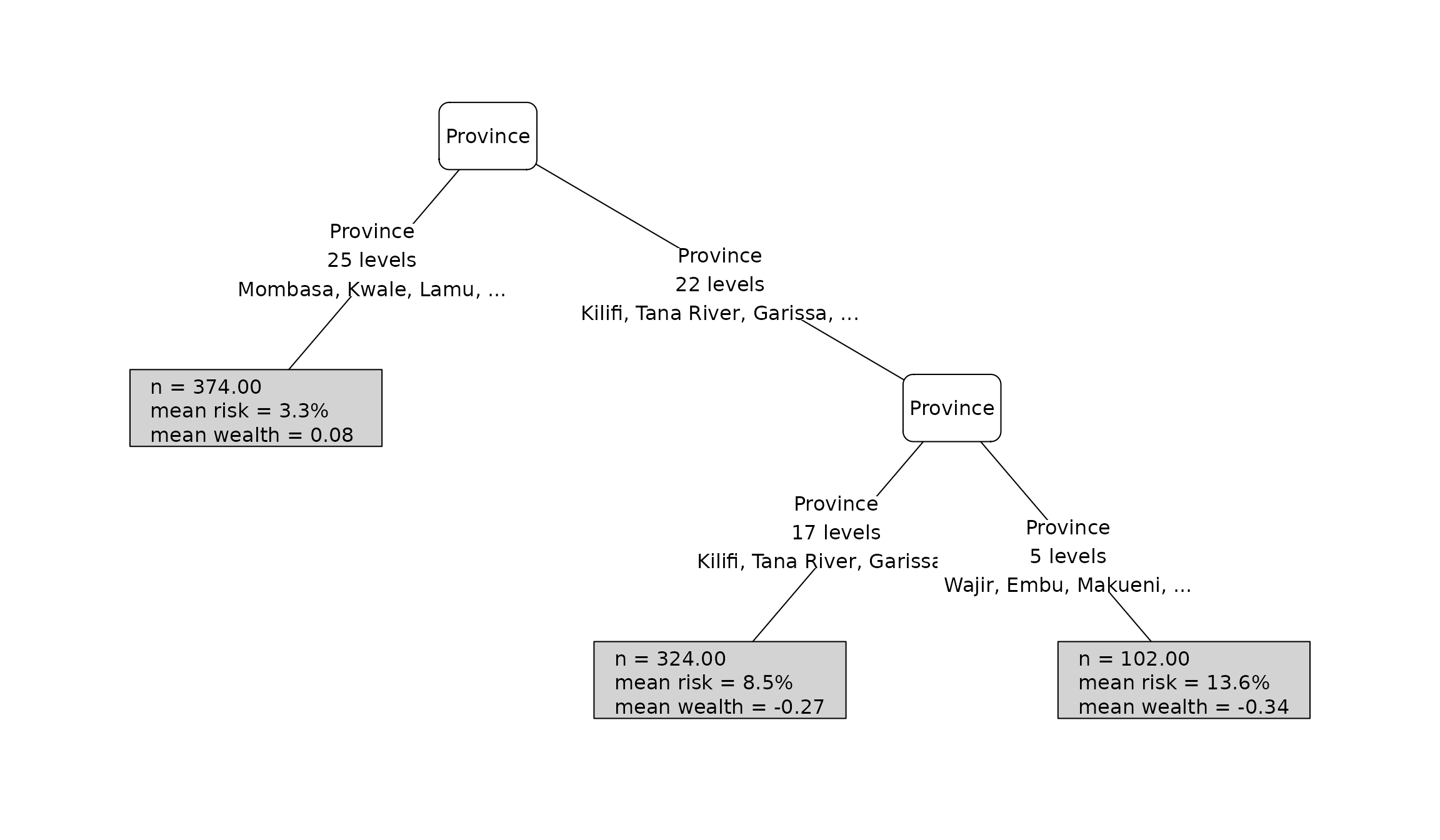
This plot should be read as a compact summary of the forest risk surface, not as a literal picture of the full ensemble.
9. Tune an inequality-aware forest with tidymodels
Forest tuning follows the same workflow logic as tree tuning. The difference is that the hyperparameter grid now spans the ensemble size, the number of candidate split variables, and the child-node size.
forest_tune_spec <- rand_forest(
  trees = tune(),
  mtry = tune(),
  min_n = tune()
) |>
  set_engine(
    "ineqTrees",
    rank_name = "wealth",
    outcome_name = "deadu5_num",
    type = "CI",
    minsplit = 120L,
    minprob = 0.05,
    maxdepth = 3L,
    min_relative_gain = tune(),
    perturb = list(replace = FALSE, fraction = 0.632)
  ) |>
  set_mode("regression")

forest_wf <- workflow() |>
  add_model(forest_tune_spec) |>
  add_formula(predictor_formula) |>
  add_case_weights(case_wt)

forest_grid <- expand.grid(
  trees = c(8L, 16L),
  mtry = c(1L, 3L),
  min_n = c(40L, 90L),
  min_relative_gain = c(0, 0.05),
  KEEP.OUT.ATTRS = FALSE,
  stringsAsFactors = FALSE
)

forest_grid
#>    trees mtry min_n min_relative_gain
#> 1      8    1    40              0.00
#> 2     16    1    40              0.00
#> 3      8    3    40              0.00
#> 4     16    3    40              0.00
#> 5      8    1    90              0.00
#> 6     16    1    90              0.00
#> 7      8    3    90              0.00
#> 8     16    3    90              0.00
#> 9      8    1    40              0.05
#> 10    16    1    40              0.05
#> 11     8    3    40              0.05
#> 12    16    3    40              0.05
#> 13     8    1    90              0.05
#> 14    16    1    90              0.05
#> 15     8    3    90              0.05
#> 16    16    3    90              0.05
set.seed(20260516)

forest_tuned <- tune_grid(
  forest_wf,
  resamples = tree_folds,
  grid = forest_grid,
  metrics = ci_tuning_metrics,
  control = control_grid(save_pred = TRUE, parallel_over = "resamples")
)

collect_metrics(forest_tuned)
#> # A tibble: 64 × 10
#>     mtry trees min_n min_relative_gain .metric  .estimator    mean     n std_err
#>    <int> <int> <int>             <dbl> <chr>    <chr>        <dbl> <int>   <dbl>
#>  1     1     8    40              0    relativ… standard    0.0269     3 0.0661
#>  2     1     8    40              0    relativ… standard   -0.295      3 0.211
#>  3     1     8    40              0    trainin… standard    0.0130     3 0.0150
#>  4     1     8    40              0    validat… standard   -0.0263     3 0.0282
#>  5     1     8    40              0.05 relativ… standard    0.0571     3 0.0127
#>  6     1     8    40              0.05 relativ… standard   -0.167      3 0.107
#>  7     1     8    40              0.05 trainin… standard    0.0134     3 0.00326
#>  8     1     8    40              0.05 validat… standard   -0.0184     3 0.0100
#>  9     1     8    90              0    relativ… standard   -0.0532     3 0.0322
#> 10     1     8    90              0    relativ… standard   -0.0396     3 0.0299
#> # ℹ 54 more rows
#> # ℹ 1 more variable: .config <chr>
show_best(forest_tuned, metric = "relative_validation_gain", n = 4)
#> # A tibble: 4 × 10
#>    mtry trees min_n min_relative_gain .metric   .estimator    mean     n std_err
#>   <int> <int> <int>             <dbl> <chr>     <chr>        <dbl> <int>   <dbl>
#> 1     1     8    90              0    relative… standard   -0.0396     3  0.0299
#> 2     1    16    40              0    relative… standard   -0.0688     3  0.0595
#> 3     1    16    90              0    relative… standard   -0.105      3  0.0840
#> 4     1     8    90              0.05 relative… standard   -0.109      3  0.0929
#> # ℹ 1 more variable: .config <chr>

best_forest <- select_best(forest_tuned, metric = "relative_validation_gain")
best_forest
#> # A tibble: 1 × 5
#>    mtry trees min_n min_relative_gain .config
#>   <int> <int> <int>             <dbl> <chr>
#> 1     1     8    90                 0 pre0_mod03_post0
The finalized workflow again contains a regular
ci_forest engine fit, so the package-native summary methods
still work after tuning.
final_forest_wf <- finalize_workflow(forest_wf, best_forest)
final_forest_fit <- fit(final_forest_wf, data = kenya_model)
final_forest_engine <- extract_fit_parsnip(final_forest_fit)$fit

ci_forest_summary(final_forest_engine)
#>    ntree  mtry   type     n mean_outcome mean_prediction outcome_ci
#>    <int> <int> <char> <int>        <num>           <num>      <num>
#> 1:     8     1     CI   800    0.0672727      0.06666129  0.2573396
#>    prediction_ci mean_terminal_nodes mean_max_depth
#>            <num>               <num>          <num>
#> 1:    0.02418404                 1.5            0.5
final_forest_pred <- predict(final_forest_fit, new_data = kenya_model)$.pred

final_forest_data <- kenya_model
final_forest_data$forest_risk <- final_forest_pred

final_forest_surrogate_spec <- decision_tree(
  tree_depth = 3L,
  min_n = 60L
) |>
  set_engine(
    "ineqTrees",
    rank_name = "wealth",
    outcome_name = "forest_risk",
    type = "CI",
    minsplit = 120L,
    minprob = 0.05,
    min_gain = 0,
    min_relative_gain = 0
  ) |>
  set_mode("regression")

final_forest_surrogate <- fit(
  final_forest_surrogate_spec,
  forest_risk ~ wealth + rural + ed + reg + unskilled,
  data = final_forest_data,
  case_weights = final_forest_data$case_wt
)

final_forest_nodes <- as.integer(predict(
  final_forest_surrogate,
  new_data = final_forest_data,
  type = "raw"
))

final_forest_gain_scores <- data.frame(
  truth = final_forest_data$deadu5_num,
  pred = final_forest_pred,
  rank = final_forest_data$wealth,
  node = final_forest_nodes,
  weight = final_forest_data$sample_weight
)

ci_gain(
  final_forest_gain_scores,
  truth = truth,
  estimate = pred,
  rank = rank,
  node = node,
  case_weights = weight,
  type = "CI"
)
#> # A tibble: 1 × 3
#>   .metric .estimator .estimate
#>   <chr>   <chr>          <dbl>
#> 1 ci_gain standard     0.00520
10. Where to go next
The tidymodels workflow covers the same modeling ideas as the package-native article, but through a different orchestration layer:
-
decision_tree()andrand_forest()define generic model controls; -
set_engine("ineqTrees", ...)supplies the inequality-specific arguments; -
fit()returns parsnip model objects whose underlying engine fits are stillci_treeandci_forestobjects; -
plot()andci_tree_terminal_summary()still work on the extracted tree fits; -
workflow(),vfold_cv(), tuning grids, andtune_grid()provide the resampling and tuning machinery; -
ci_gain()can be used both as the tuning metric and as the final concentration-index interpretation.
If you want the most direct concentration-index tuning workflow, the
package helpers such as tune_ci_tree() and
tune_ci_forest() are still the most natural choice. If you
want model specifications, workflows, and resampling to live inside
tidymodels, the bridge shown here keeps that option open without giving
up the interpretation tools already built into
ineqTrees.