tidmodels_ineqTrees

library(ineqTrees)

Introduction

This article shows how to fit ineqTrees models from the tidymodels framework. The core idea is still the same as in the package-native API: the model needs a socioeconomic rank, an outcome, and predictors that define subgroups. The tidymodels bridge lets those pieces move through parsnip, workflows, rsample, dials, and tune.

The examples use the simulated kenya data shipped with the package. We fit:

a single concentration-index decision tree;
a single concentration-index forest;
plots for the fitted tree and an interpretable forest surrogate;
tuned tree and forest workflows using tune::tune_grid().

1. Load packages and data

This chunk loads the modeling packages used in the article. ineqTrees registers its parsnip engines on load, and register_ineqtrees_parsnip() is called explicitly so the code is clear when copied into a fresh session.

library(ineqTrees)
library(parsnip)
library(workflows)
library(rsample)
library(dials)
#> Loading required package: scales
library(tune)
library(yardstick)
library(hardhat)
library(data.table)
#> 
#> Attaching package: 'data.table'
#> The following object is masked from 'package:base':
#> 
#>     %notin%

register_ineqtrees_parsnip()

data(kenya, package = "ineqTrees")
setDT(kenya)

2. Prepare a tidymodels analysis table

This chunk keeps the rank, outcome, predictors, and survey weight in one complete analysis table. We then add case_wt, a hardhat importance-weight column that workflows can pass into parsnip during fitting and tuning.

analysis_vars <- c(
  "wealth",
  "deadu5_num",
  "rural",
  "ed",
  "reg",
  "unskilled",
  "sample_weight"
)

kenya_model <- kenya[
  complete.cases(kenya[, ..analysis_vars]),
  ..analysis_vars
]

set.seed(20260513)
kenya_model <- as.data.frame(kenya_model[
  sample.int(.N, min(600L, .N))
])

kenya_model$case_wt <- hardhat::importance_weights(kenya_model$sample_weight)

predictor_formula <- deadu5_num ~ wealth + rural + ed + reg + unskilled

head(kenya_model[, c("wealth", "deadu5_num", "rural", "ed", "case_wt")])
#>        wealth deadu5_num rural             ed   case_wt
#> 1 -0.16385206          0 Rural    a education 0.1952118
#> 2 -0.40154035          0 Urban    a education 5.0486062
#> 3 -0.86970946          1 Rural    a education 1.2777867
#> 4 -1.08425705          0 Rural b no education 0.2530733
#> 5 -0.04800034          0 Rural    a education 0.7291354
#> 6 -0.70405442          0 Urban b no education 1.2659496

The formula includes wealth on the right-hand side only so tidymodels keeps the rank column available to the engine. The ineqTrees bridge removes wealth from the split predictors internally and uses it as rank_name.

3. Fit a single CI decision tree

This chunk builds a parsnip decision-tree specification. The generic tidymodels arguments map to ineqTrees controls: tree_depth maps to maximum depth and min_n maps to the child-node size. Inequality-specific settings, such as rank_name, outcome_name, and type, are supplied through set_engine().

tree_spec <- decision_tree(
  tree_depth = 3L,
  min_n = 60L
) |>
  set_engine(
    "ineqTrees",
    rank_name = "wealth",
    outcome_name = "deadu5_num",
    type = "CI",
    minsplit = 120L,
    minprob = 0.05,
    min_gain = 0
  ) |>
  set_mode("regression")

tree_spec
#> Decision Tree Model Specification (regression)
#> 
#> Main Arguments:
#>   tree_depth = 3
#>   min_n = 60
#> 
#> Engine-Specific Arguments:
#>   rank_name = wealth
#>   outcome_name = deadu5_num
#>   type = CI
#>   minsplit = 120
#>   minprob = 0.05
#>   min_gain = 0
#> 
#> Computational engine: ineqTrees

This chunk fits the tree. The formula is the tidymodels-style single-outcome formula; the bridge rebuilds the two-column cbind(wealth, deadu5_num) response before calling ci_tree().

tree_fit <- fit(
  tree_spec,
  predictor_formula,
  data = kenya_model,
  case_weights = kenya_model$case_wt
)

tree_fit$fit

Greedy concentration-index tree

Formula: cbind(wealth, deadu5_num) ~ rural + ed + reg + unskilled Criterion: CI Tree size: 3 inner nodes, 4 terminal nodes, max depth 3

Terminal-node summary with subgroup rules
node	n	weight	depth	CI	outcome_mean	outcome_percent	rule
7	150	121.49903	2	0.357	0.215	21.5	reg in {Mombasa, Kwale, Tana River, Taita Taveta, Garissa, Wajir, Marsabit, Isiolo, Meru, Machakos, Makueni, Nyeri, Murang’a, Kiambu, Turkana, Samburu, Uasin Gishu, Nandi, Baringo, Nakuru, Narok, Kakamega, Bungoma, Siaya, Kisumu, Homa Bay, Migori, Kisii, Nyamira} & reg in {Kwale, Taita Taveta, Garissa, Marsabit, Isiolo, Makueni, Nyeri, Murang’a, Turkana, Nandi, Nakuru, Siaya}
6	94	77.41979	3	0.206	0.106	10.6	reg in {Mombasa, Kwale, Tana River, Taita Taveta, Garissa, Wajir, Marsabit, Isiolo, Meru, Machakos, Makueni, Nyeri, Murang’a, Kiambu, Turkana, Samburu, Uasin Gishu, Nandi, Baringo, Nakuru, Narok, Kakamega, Bungoma, Siaya, Kisumu, Homa Bay, Migori, Kisii, Nyamira} & reg in {Mombasa, Tana River, Wajir, Meru, Machakos, Kiambu, Samburu, Uasin Gishu, Baringo, Narok, Kakamega, Bungoma, Kisumu, Homa Bay, Migori, Kisii, Nyamira} & unskilled in {Yes}
5	178	174.28762	3	0.023	0.056	5.6	reg in {Mombasa, Kwale, Tana River, Taita Taveta, Garissa, Wajir, Marsabit, Isiolo, Meru, Machakos, Makueni, Nyeri, Murang’a, Kiambu, Turkana, Samburu, Uasin Gishu, Nandi, Baringo, Nakuru, Narok, Kakamega, Bungoma, Siaya, Kisumu, Homa Bay, Migori, Kisii, Nyamira} & reg in {Mombasa, Tana River, Wajir, Meru, Machakos, Kiambu, Samburu, Uasin Gishu, Baringo, Narok, Kakamega, Bungoma, Kisumu, Homa Bay, Migori, Kisii, Nyamira} & unskilled in {No}
2	178	152.05176	1	0.000	0.000	0.0	reg in {Kilifi, Lamu, Mandera, Tharaka-Nithi, Embu, Kitui, Nyandarua, Kirinyaga, West Pokot, Trans Nzoia, Elgeyo-Marakwet, Laikipia, Kajiado, Kericho, Bomet, Vihiga, Busia, Nairobi}

This chunk creates fitted risks and terminal-node ids. Numeric predictions are returned as a tibble with .pred; raw predictions return the terminal node partition used for concentration-index gain.

tree_pred <- predict(tree_fit, new_data = kenya_model)
tree_nodes <- predict(tree_fit, new_data = kenya_model, type = "raw")

tree_scores <- data.frame(
  truth = kenya_model$deadu5_num,
  pred = tree_pred$.pred,
  rank = kenya_model$wealth,
  node = tree_nodes,
  weight = kenya_model$sample_weight
)

ci_gain(
  tree_scores,
  truth = truth,
  estimate = pred,
  rank = rank,
  node = node,
  case_weights = weight,
  type = "CI"
)
#> # A tibble: 1 × 3
#>   .metric .estimator .estimate
#>   <chr>   <chr>          <dbl>
#> 1 ci_gain standard       0.207

4. Plot the fitted tree

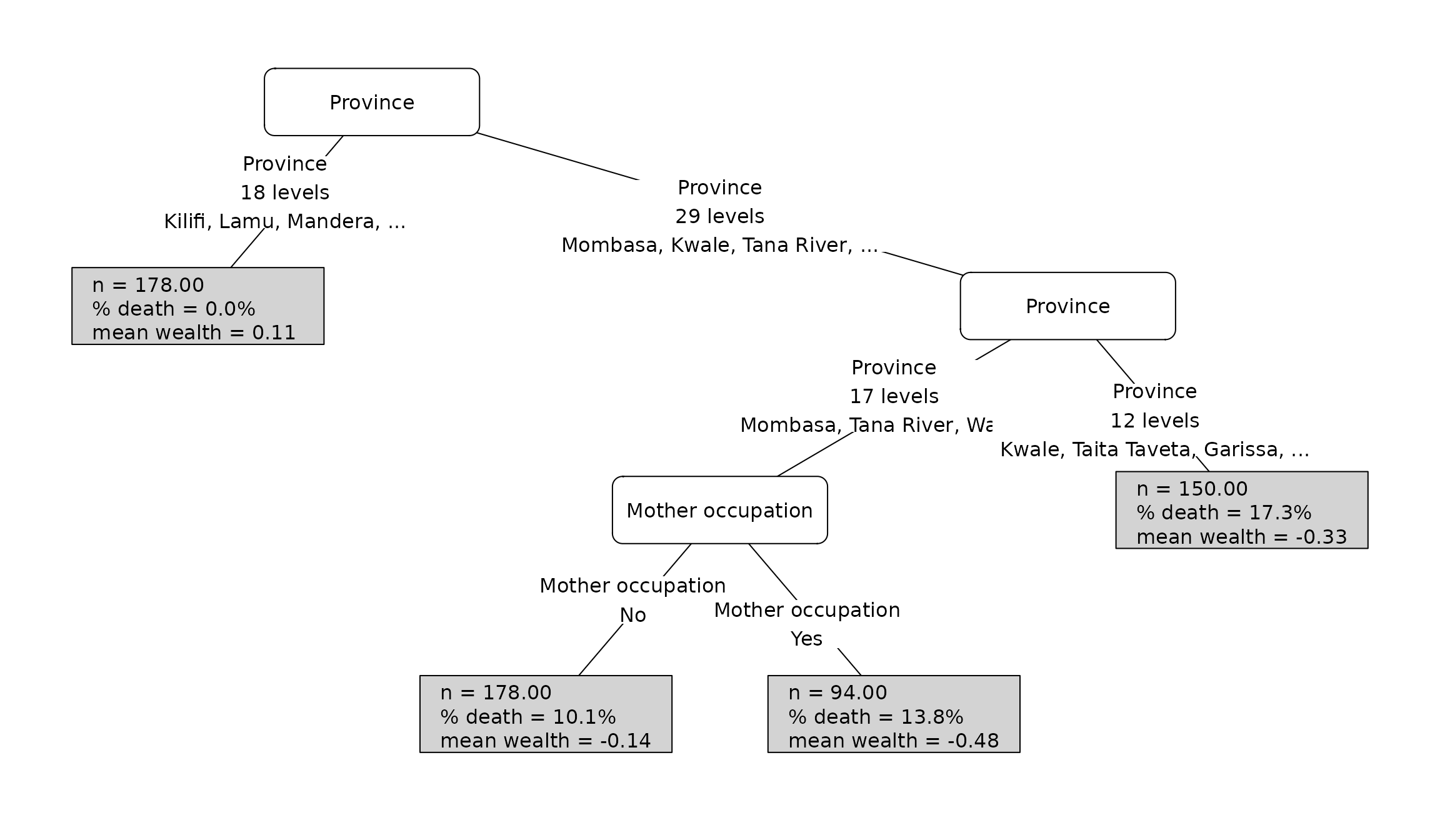
This chunk plots the fitted ci_tree stored inside the parsnip fit. The plot method comes from ineqTrees and partykit, so we can use the same reporting options as package-native ci_tree() fits.

plot(
  tree_fit$fit,
  data = kenya_model,
  var_labels = c(
    rural = "Residence",
    ed = "Mother education",
    reg = "Province",
    unskilled = "Mother occupation"
  ),
  terminal_stats = list(
    n = nrow,
    mortality = function(df) mean(df$deadu5_num),
    mean_wealth = function(df) mean(df$wealth)
  ),
  stat_labels = c(
    n = "n",
    mortality = "% death",
    mean_wealth = "mean wealth"
  ),
  stat_formatters = list(
    mortality = function(x) sprintf("%.1f%%", 100 * x),
    mean_wealth = function(x) sprintf("%.2f", x)
  )
)

A concentration-index decision tree fitted through parsnip.

5. Fit a single CI forest

This chunk builds a random-forest specification. The generic tidymodels arguments map to forest controls: trees maps to ntree, mtry controls the number of candidate split variables, and min_n maps to minbucket.

forest_spec <- rand_forest(
  trees = 20L,
  mtry = 2L,
  min_n = 60L
) |>
  set_engine(
    "ineqTrees",
    rank_name = "wealth",
    outcome_name = "deadu5_num",
    type = "CI",
    minsplit = 120L,
    minprob = 0.05,
    maxdepth = 3L,
    perturb = list(replace = FALSE, fraction = 0.632)
  ) |>
  set_mode("regression")

forest_spec
#> Random Forest Model Specification (regression)
#> 
#> Main Arguments:
#>   mtry = 2
#>   trees = 20
#>   min_n = 60
#> 
#> Engine-Specific Arguments:
#>   rank_name = wealth
#>   outcome_name = deadu5_num
#>   type = CI
#>   minsplit = 120
#>   minprob = 0.05
#>   maxdepth = 3
#>   perturb = list(replace = FALSE, fraction = 0.632)
#> 
#> Computational engine: ineqTrees

This chunk fits the forest through parsnip and prints a compact summary of the underlying ci_forest object.

set.seed(20260513)

forest_fit <- fit(
  forest_spec,
  predictor_formula,
  data = kenya_model,
  case_weights = kenya_model$case_wt
)

ci_forest_summary(forest_fit$fit)
#>    ntree  mtry   type     n mean_outcome mean_prediction outcome_ci
#>    <int> <int> <char> <int>        <num>           <num>      <num>
#> 1:    20     2     CI   600   0.08394269       0.0790194  0.3278152
#>    prediction_ci mean_terminal_nodes mean_max_depth
#>            <num>               <num>          <num>
#> 1:    0.07715226                 2.8           1.65

This chunk predicts from the forest and measures inequality in the fitted risks. This is not validation gain; it is the concentration index of the forest’s predicted outcome.

forest_pred <- predict(forest_fit, new_data = kenya_model)

forest_scores <- data.frame(
  truth = kenya_model$deadu5_num,
  pred = forest_pred$.pred,
  rank = kenya_model$wealth,
  weight = kenya_model$sample_weight
)

ci_prediction_index(
  forest_scores,
  truth = truth,
  estimate = pred,
  rank = rank,
  case_weights = weight,
  type = "CI"
)
#> # A tibble: 1 × 3
#>   .metric             .estimator .estimate
#>   <chr>               <chr>          <dbl>
#> 1 ci_prediction_index standard      0.0777

6. Plot the forest with a surrogate tree

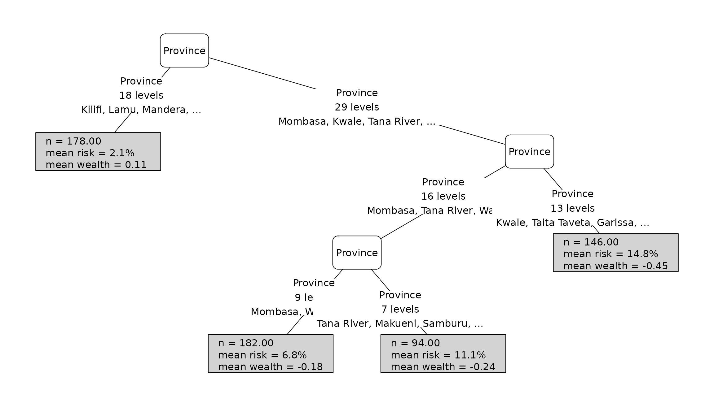
A forest is an ensemble, so there is no single tree plot that fully describes the model. This chunk fits a small surrogate CI tree to the forest predictions. The surrogate is useful for communicating the main subgroup structure in the forest risk surface.

surrogate_data <- kenya_model
surrogate_data$forest_risk <- forest_pred$.pred

surrogate_spec <- decision_tree(
  tree_depth = 3L,
  min_n = 60L
) |>
  set_engine(
    "ineqTrees",
    rank_name = "wealth",
    outcome_name = "forest_risk",
    type = "CI",
    minsplit = 120L,
    minprob = 0.05
  ) |>
  set_mode("regression")

surrogate_fit <- fit(
  surrogate_spec,
  forest_risk ~ wealth + rural + ed + reg + unskilled,
  data = surrogate_data,
  case_weights = surrogate_data$case_wt
)

ci_tree_terminal_summary(surrogate_fit$fit)[
  ,
  c("node", "n", "ci", "outcome_mean", "rule")
]
#>     node     n          ci outcome_mean
#>    <int> <int>       <num>        <num>
#> 1:     2   178 0.021434368   0.02087096
#> 2:     5   182 0.003523024   0.06759835
#> 3:     6    94 0.001620644   0.10964072
#> 4:     7   146 0.012418661   0.14662473
#>                                                                                                                                                                                                                                                                                                                                                                                                                                                                                                                 rule
#>                                                                                                                                                                                                                                                                                                                                                                                                                                                                                                               <char>
#> 1:                                                                                                                                                                                                                                                                                                                             reg in {Kilifi, Lamu, Mandera, Tharaka-Nithi, Embu, Kitui, Nyandarua, Kirinyaga, West Pokot, Trans Nzoia, Elgeyo-Marakwet, Laikipia, Kajiado, Kericho, Bomet, Vihiga, Busia, Nairobi}
#> 2: reg in {Mombasa, Kwale, Tana River, Taita Taveta, Garissa, Wajir, Marsabit, Isiolo, Meru, Machakos, Makueni, Nyeri, Murang'a, Kiambu, Turkana, Samburu, Uasin Gishu, Nandi, Baringo, Nakuru, Narok, Kakamega, Bungoma, Siaya, Kisumu, Homa Bay, Migori, Kisii, Nyamira} & reg in {Mombasa, Tana River, Wajir, Meru, Machakos, Makueni, Kiambu, Samburu, Baringo, Nakuru, Narok, Kakamega, Bungoma, Kisumu, Homa Bay, Nyamira} & reg in {Mombasa, Wajir, Meru, Machakos, Kiambu, Narok, Kakamega, Bungoma, Kisumu}
#> 3:         reg in {Mombasa, Kwale, Tana River, Taita Taveta, Garissa, Wajir, Marsabit, Isiolo, Meru, Machakos, Makueni, Nyeri, Murang'a, Kiambu, Turkana, Samburu, Uasin Gishu, Nandi, Baringo, Nakuru, Narok, Kakamega, Bungoma, Siaya, Kisumu, Homa Bay, Migori, Kisii, Nyamira} & reg in {Mombasa, Tana River, Wajir, Meru, Machakos, Makueni, Kiambu, Samburu, Baringo, Nakuru, Narok, Kakamega, Bungoma, Kisumu, Homa Bay, Nyamira} & reg in {Tana River, Makueni, Samburu, Baringo, Nakuru, Homa Bay, Nyamira}
#> 4:                                                                                                             reg in {Mombasa, Kwale, Tana River, Taita Taveta, Garissa, Wajir, Marsabit, Isiolo, Meru, Machakos, Makueni, Nyeri, Murang'a, Kiambu, Turkana, Samburu, Uasin Gishu, Nandi, Baringo, Nakuru, Narok, Kakamega, Bungoma, Siaya, Kisumu, Homa Bay, Migori, Kisii, Nyamira} & reg in {Kwale, Taita Taveta, Garissa, Marsabit, Isiolo, Nyeri, Murang'a, Turkana, Uasin Gishu, Nandi, Siaya, Migori, Kisii}

This chunk plots the surrogate tree. Read it as a summary of the forest’s predicted risk pattern, not as the forest itself.

plot(
  surrogate_fit$fit,
  data = surrogate_data,
  var_labels = c(
    rural = "Residence",
    ed = "Mother education",
    reg = "Province",
    unskilled = "Mother occupation"
  ),
  terminal_stats = list(
    n = nrow,
    mean_risk = function(df) mean(df$forest_risk),
    mean_wealth = function(df) mean(df$wealth)
  ),
  stat_labels = c(
    n = "n",
    mean_risk = "mean risk",
    mean_wealth = "mean wealth"
  ),
  stat_formatters = list(
    mean_risk = function(x) sprintf("%.1f%%", 100 * x),
    mean_wealth = function(x) sprintf("%.2f", x)
  )
)

A surrogate concentration-index tree for forest predictions.

7. Tune a CI tree with `tune`

This chunk creates resamples. Because the outcome is binary, stratifying by deadu5_num helps keep events distributed across folds.

set.seed(20260513)

folds <- vfold_cv(
  kenya_model,
  v = 3L,
  strata = deadu5_num
)

folds
#> #  3-fold cross-validation using stratification 
#> # A tibble: 3 × 2
#>   splits            id   
#>   <list>            <chr>
#> 1 <split [400/200]> Fold1
#> 2 <split [400/200]> Fold2
#> 3 <split [400/200]> Fold3

This chunk creates a tunable tree specification. tree_depth and min_n are marked with tune(), while the inequality-specific engine arguments remain fixed for this search.

tree_tune_spec <- decision_tree(
  tree_depth = tune(),
  min_n = tune()
) |>
  set_engine(
    "ineqTrees",
    rank_name = "wealth",
    outcome_name = "deadu5_num",
    type = "CI",
    minsplit = 120L,
    minprob = 0.05
  ) |>
  set_mode("regression")

This chunk combines the model, formula, and case weights into a workflow. Again, wealth is present in the formula to carry the rank through tidymodels; the bridge removes it from the split predictors before fitting.

tree_wf <- workflow() |>
  add_model(tree_tune_spec) |>
  add_formula(predictor_formula) |>
  add_case_weights(case_wt)

tree_wf
#> ══ Workflow ════════════════════════════════════════════════════════════════════
#> Preprocessor: Formula
#> Model: decision_tree()
#> 
#> ── Preprocessor ────────────────────────────────────────────────────────────────
#> deadu5_num ~ wealth + rural + ed + reg + unskilled
#> 
#> ── Case Weights ────────────────────────────────────────────────────────────────
#> case_wt
#> 
#> ── Model ───────────────────────────────────────────────────────────────────────
#> Decision Tree Model Specification (regression)
#> 
#> Main Arguments:
#>   tree_depth = tune()
#>   min_n = tune()
#> 
#> Engine-Specific Arguments:
#>   rank_name = wealth
#>   outcome_name = deadu5_num
#>   type = CI
#>   minsplit = 120
#>   minprob = 0.05
#> 
#> Computational engine: ineqTrees

This chunk defines a small tuning grid. Larger applied analyses can expand the ranges or use grid_latin_hypercube() for a broader search.

tree_grid <- grid_regular(
  tree_depth(range = c(2L, 4L)),
  min_n(range = c(40L, 90L)),
  levels = 2L
)

tree_grid
#> # A tibble: 4 × 2
#>   tree_depth min_n
#>        <int> <int>
#> 1          2    40
#> 2          4    40
#> 3          2    90
#> 4          4    90

This chunk runs cross-validation with tune_grid(). The model is still an inequality-aware tree; here the tuning metric is prediction error, which is what tune_grid() can compute directly from .pred and the observed outcome.

set.seed(20260513)

tree_tuned <- tune_grid(
  tree_wf,
  resamples = folds,
  grid = tree_grid,
  metrics = metric_set(rmse, mae),
  control = control_grid(save_pred = TRUE)
)

collect_metrics(tree_tuned)
#> # A tibble: 8 × 8
#>   tree_depth min_n .metric .estimator  mean     n std_err .config        
#>        <int> <int> <chr>   <chr>      <dbl> <int>   <dbl> <chr>          
#> 1          2    40 mae     standard   0.160     3 0.00142 pre0_mod1_post0
#> 2          2    40 rmse    standard   0.308     3 0.0124  pre0_mod1_post0
#> 3          2    90 mae     standard   0.159     3 0.00634 pre0_mod2_post0
#> 4          2    90 rmse    standard   0.304     3 0.0146  pre0_mod2_post0
#> 5          4    40 mae     standard   0.161     3 0.00173 pre0_mod3_post0
#> 6          4    40 rmse    standard   0.309     3 0.0131  pre0_mod3_post0
#> 7          4    90 mae     standard   0.159     3 0.00645 pre0_mod4_post0
#> 8          4    90 rmse    standard   0.303     3 0.0140  pre0_mod4_post0

This chunk selects the best tree by RMSE and refits it on the full analysis table. The resulting workflow can be predicted from like any other tidymodels fit.

best_tree <- select_best(tree_tuned, metric = "rmse")

final_tree_wf <- finalize_workflow(tree_wf, best_tree)
final_tree_fit <- fit(final_tree_wf, data = kenya_model)

best_tree
#> # A tibble: 1 × 3
#>   tree_depth min_n .config        
#>        <int> <int> <chr>          
#> 1          4    90 pre0_mod4_post0

8. Tune a CI forest with `tune`

This chunk creates a tunable forest specification. Forest tuning usually searches over the ensemble size, mtry, and the child-node size.

forest_tune_spec <- rand_forest(
  trees = tune(),
  mtry = tune(),
  min_n = tune()
) |>
  set_engine(
    "ineqTrees",
    rank_name = "wealth",
    outcome_name = "deadu5_num",
    type = "CI",
    minsplit = 120L,
    minprob = 0.05,
    maxdepth = 3L,
    perturb = list(replace = FALSE, fraction = 0.632)
  ) |>
  set_mode("regression")

This chunk wraps the forest specification in a workflow. The formula and case weights are the same as for the tree workflow.

forest_wf <- workflow() |>
  add_model(forest_tune_spec) |>
  add_formula(predictor_formula) |>
  add_case_weights(case_wt)

This chunk defines a deliberately small forest grid so the article builds quickly. Increase trees, add more levels, or use randomized grids for a final analysis.

forest_grid <- grid_regular(
  trees(range = c(8L, 16L)),
  mtry(range = c(1L, 3L)),
  min_n(range = c(40L, 90L)),
  levels = 2L
)

forest_grid
#> # A tibble: 8 × 3
#>   trees  mtry min_n
#>   <int> <int> <int>
#> 1     8     1    40
#> 2    16     1    40
#> 3     8     3    40
#> 4    16     3    40
#> 5     8     1    90
#> 6    16     1    90
#> 7     8     3    90
#> 8    16     3    90

This chunk tunes the forest. The result has the standard tune_results interface, so collect_metrics(), collect_predictions(), select_best(), and show_best() work as expected.

set.seed(20260514)

forest_tuned <- tune_grid(
  forest_wf,
  resamples = folds,
  grid = forest_grid,
  metrics = metric_set(rmse, mae),
  control = control_grid(save_pred = TRUE, parallel_over = "resamples")
)

collect_metrics(forest_tuned)
#> # A tibble: 16 × 9
#>     mtry trees min_n .metric .estimator  mean     n std_err .config        
#>    <int> <int> <int> <chr>   <chr>      <dbl> <int>   <dbl> <chr>          
#>  1     1     8    40 mae     standard   0.160     3 0.00265 pre0_mod1_post0
#>  2     1     8    40 rmse    standard   0.295     3 0.0170  pre0_mod1_post0
#>  3     1     8    90 mae     standard   0.163     3 0.00889 pre0_mod2_post0
#>  4     1     8    90 rmse    standard   0.294     3 0.0163  pre0_mod2_post0
#>  5     1    16    40 mae     standard   0.160     3 0.00510 pre0_mod3_post0
#>  6     1    16    40 rmse    standard   0.294     3 0.0172  pre0_mod3_post0
#>  7     1    16    90 mae     standard   0.161     3 0.00601 pre0_mod4_post0
#>  8     1    16    90 rmse    standard   0.293     3 0.0170  pre0_mod4_post0
#>  9     3     8    40 mae     standard   0.161     3 0.00521 pre0_mod5_post0
#> 10     3     8    40 rmse    standard   0.298     3 0.0164  pre0_mod5_post0
#> 11     3     8    90 mae     standard   0.160     3 0.00463 pre0_mod6_post0
#> 12     3     8    90 rmse    standard   0.297     3 0.0178  pre0_mod6_post0
#> 13     3    16    40 mae     standard   0.159     3 0.00538 pre0_mod7_post0
#> 14     3    16    40 rmse    standard   0.299     3 0.0156  pre0_mod7_post0
#> 15     3    16    90 mae     standard   0.159     3 0.00608 pre0_mod8_post0
#> 16     3    16    90 rmse    standard   0.299     3 0.0177  pre0_mod8_post0

This chunk selects and refits the best forest. The refitted object is a workflow whose parsnip fit contains the underlying ci_forest.

best_forest <- select_best(forest_tuned, metric = "rmse")

final_forest_wf <- finalize_workflow(forest_wf, best_forest)
final_forest_fit <- fit(final_forest_wf, data = kenya_model)

best_forest
#> # A tibble: 1 × 4
#>    mtry trees min_n .config        
#>   <int> <int> <int> <chr>          
#> 1     1    16    90 pre0_mod4_post0

This chunk extracts the fitted ci_forest from the final workflow and prints the package-native forest summary.

final_forest_engine <- extract_fit_parsnip(final_forest_fit)$fit

ci_forest_summary(final_forest_engine)
#>    ntree  mtry   type     n mean_outcome mean_prediction outcome_ci
#>    <int> <int> <char> <int>        <num>           <num>      <num>
#> 1:    16     1     CI   600   0.08394269      0.08178389  0.3278152
#>    prediction_ci mean_terminal_nodes mean_max_depth
#>            <num>               <num>          <num>
#> 1:    0.04921653              1.8125         0.8125

9. Notes on tuning metrics

The ineqTrees engine optimizes concentration-index impurity while fitting. The tune package then chooses hyperparameters from the predictions it collects across resamples. Standard yardstick metrics such as RMSE and MAE work directly in tune_grid().

Exact CI validation gain needs a terminal-node partition in addition to .pred. For a single fitted tree, obtain that partition with:

head(predict(tree_fit, new_data = kenya_model, type = "raw"))
#> 1 2 3 4 5 6 
#> 2 7 6 2 7 7

Then pass those node ids to ci_gain(), as shown earlier. For forests, raw node predictions return one terminal-node column per tree, so a surrogate tree is often easier to use when you want a single interpretable partition.