library(plotly)
library(tidyverse)
library(data.table)
library(sf)
library(DT)
library(tmap)
library(rKenyaCensus)Kenya Census Data
# kenya_5yr_births <- readGoogleSheet("https://docs.google.com/spreadsheets/d/e/2PACX-1vSf-yNXNk68cIOH0Rb6alaDk9SxKEMm3h6kb2p8jxT8oMdfj4OqUDbs2Ln9OOGGCI9V7SNiZJCDWm4H/pubhtml")
#
# kenya_5yr_births <- cleanGoogleTable(kenya_5yr_births , table = 1, skip = 1 ) %>%
# setDT()
data(V4_T2.40)
kenya_5yr_births = V4_T2.40
setDT(kenya_5yr_births)old_nms_births <- names(kenya_5yr_births)
new_nms_births <- gsub("\\s", "_", old_nms_births) %>%
tolower()
setnames(kenya_5yr_births, old_nms_births, new_nms_births)numerics_nms <- c("total", "notified", "not_notified",
"don’t_know", "not_stated", "percent_notified")
kenya_5yr_births[, (numerics_nms) := lapply(.SD, function(x) gsub(",", "", x)), .SDcols = numerics_nms]
kenya_5yr_births[, (numerics_nms) := lapply(.SD, as.numeric), .SDcols = numerics_nms]kenya_counties <- st_read("County")Reading layer `County' from data source
`/home/mburu/r_projects/m-mburu.github.io/kenya_population/County'
using driver `ESRI Shapefile'
Simple feature collection with 47 features and 8 fields
Geometry type: MULTIPOLYGON
Dimension: XY
Bounding box: xmin: 33.91182 ymin: -4.702271 xmax: 41.90626 ymax: 5.430648
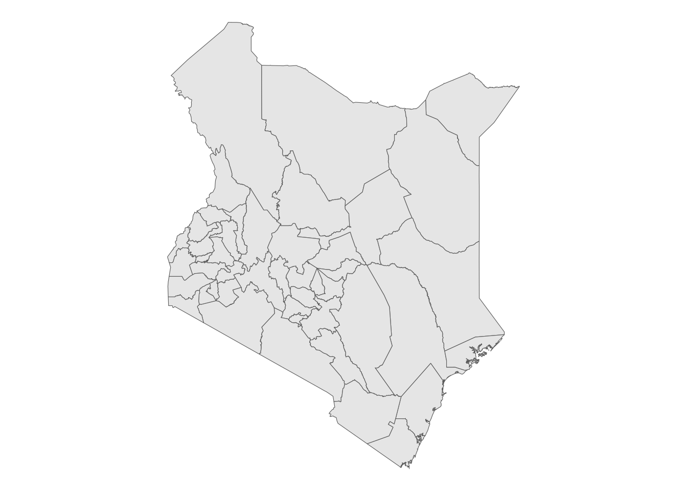
Geodetic CRS: WGS 84ggplot(kenya_counties)+
geom_sf() +
theme_void()
setnames(kenya_counties, "COUNTY", "county")kenya_5yr_births[, county := tolower(gsub("\\s", "-", county))]
kenya_5yr_births[county == "elgeyo-marakwet", county := "keiyo-marakwet" ]
kenya_5yr_births[county == "nairobi-city" , county := "nairobi"]
kenya_5yr_births[county == "tharaka-nithi" , county := "tharaka" ]
kenya_5yr_births[county == "homabay" , county := "homa-bay" ]
setDT(kenya_counties)
kenya_counties[, county := tolower(gsub("\\s", "-", county))]
kenya_births_counties <- merge(kenya_counties, kenya_5yr_births, by = "county" )
setnames(kenya_births_counties, "percent_notified", "per_cent_in_health_facility")
kenya_births_counties[, county := paste(county, " ", per_cent_in_health_facility,"%", sep = "" )]
kenya_births_counties <- st_set_geometry(kenya_births_counties, "geometry")map1 <- tm_shape(kenya_births_counties)+
tm_borders(col = "gold")+
tm_polygons(col = "per_cent_in_health_facility")+
tm_layout(title = "% Health facility births",
title.position = c(0.3, "top"))
tmap_leaflet(map1)kenyan_pop <- fread("distribution-of-population-by-age-and-sex-kenya-2019-census-volume-iii.csv")numerics_nms <- c("Male", "Female", "Intersex")
kenyan_pop[, (numerics_nms) := lapply(.SD, function(x) gsub(",", "", x)), .SDcols = numerics_nms]
kenyan_pop[, (numerics_nms) := lapply(.SD, as.numeric), .SDcols = numerics_nms]
kenyan_pop[, (numerics_nms) := lapply(.SD, function(x) ifelse(is.na(x), 0, x)), .SDcols = numerics_nms]
kenyan_pop[, Age := gsub("Sep", "09", Age)]
kenyan_pop[, Age := gsub("Oct", "10", Age)]
kenyan_pop[,Total:= Reduce(`+`, .SD),.SDcols= numerics_nms]age_cat <- kenyan_pop[!grepl("-", Age)]
age_cat[is.na(age_cat)] <- NA
#age_cat[,Total:= Reduce(`+`, .SD),.SDcols= numerics_nms]age_cat_m <- melt(age_cat, id.vars = c("Age", "Total"), variable.name = "Sex")
age_cat_m[, Perc := round(value/Total*100, 2)]library(ggthemes)
age_cat_m <- age_cat_m[Age != "Total"]
age_cat_m[, Age := as.numeric(Age)]
pop_plot <- ggplot(age_cat_m, aes(Age, Perc, group = Sex))+
geom_line(aes(color = Sex)) +
labs(y = "Percentage of Population")+
scale_x_continuous(breaks = seq(0, 100, by = 10))+
scale_color_viridis_d()+
theme_hc()
ggplotly(pop_plot)age_cat[is.na(Age), Age := 100]
age_cat[, Age := as.numeric(Age)]
age_cat[, age_factor := cut(Age,
breaks = c(0, 5, 15, 20, 30, 40, 50, 65, 100 ),
include.lowest = T,
labels = c("0-5", "6-15", "16-20",
"20-30", "31-40", "41,50]",
"51-65", "> 65"))]
age_cat_sum <- age_cat[, .(sum_total = sum(Total)), by = age_factor] %>%
.[, Perc := round(sum_total/sum(sum_total)*100,2)]Age Summary Stats
age_cat <- age_cat[!is.na(Age)]
list_df <- list()
for (i in 1:nrow(age_cat)) {
list_df[[i]]<- data.table (Age = rep(age_cat[i,Age], age_cat[i, Total]))
}
dt_age <- rbindlist(list_df)
dt_age[, .(Mean = round(mean(Age),1),
Median = median(Age),
First_quartile = quantile(Age, 0.25),
Third_quartile = quantile(Age, 0.75))] %>%
datatable()library(scales)
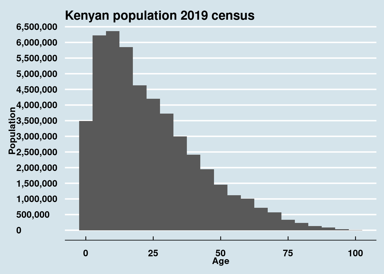
ggplot(dt_age, aes(Age)) +
geom_histogram(binwidth = 5) +
labs(y = "Population")+
theme_economist()+
scale_y_continuous(label=comma, breaks = seq(from = 0, to = 6500000, by = 500000))+
labs(title = "Kenyan population 2019 census")+
theme(
axis.text = element_text(size =12, face = "bold"),
axis.title = element_text(size =12, face = "bold"))
#ggplotly(pop_plot2)library(knitr)
crops <-fread("distribution-of-households-growing-other-crops-by-type-county-and-sub-county-2019-census-volume-.csv")
setnames(crops, "County/Sub County", "county")
crops_m <- melt(crops, id.vars = c("county", "Farming"),
variable.factor = F, variable.name = "crops",
value.name = "households")
nms <- c("Farming", "households")
crops_m[, (nms) := lapply(.SD, function(x) gsub(",", "", x)), .SDcols = nms]
crops_m[, (nms) := lapply(.SD, as.numeric), .SDcols = nms]
crops_m[, (nms) := lapply(.SD, function(x) ifelse(is.na(x), 0, x)), .SDcols = nms]
crops_m[, Perc := round(households/Farming * 100, 2)]
set.seed(100)
crops_m[sample(1:nrow(crops_m),20)] %>% datatable()kenya_crops <-crops_m[county == "KENYA"]
setorder(kenya_crops, -Perc)
datatable(kenya_crops)crops_bar <- ggplot(kenya_crops, aes(reorder(crops, Perc), Perc))+
geom_bar(stat = "identity")+
theme_economist()+
labs(y = "Percentage of households", x = "Crops",
title = "Percentage of Kenyan households growing crops")+
theme_hc()+
coord_flip()
ggplotly(crops_bar)#crops_m[, county := tolower(county)]
crops_m[, county := tolower(gsub("\\s", "-", county))]
crops_m[county == "elgeyo/marakwet", county := "keiyo-marakwet"]
crops_m[county == "tharaka---nithi", county := "tharaka"]
crops_m[county == "taita/taveta", county := "taita-taveta"]
crops_counties_dat <- merge(crops_m, kenya_counties, by = "county")
farm <- unique(crops_counties_dat, by = c("county","Farming"))
farm <- farm %>% group_by(county) %>%
filter(Farming == max(Farming)) %>%
setDT()
crops_counties_dat <- merge(crops_counties_dat,
farm[, .(county, Farming)],
by = c("county", "Farming"))
pop_crops_counties <- crops_counties_dat %>%
group_by(county) %>%
filter(Perc == max(Perc)) %>%
ungroup()%>%
mutate(county = paste0(county," ", crops," ", Perc, "%"))
pop_crops_counties <- st_set_geometry(pop_crops_counties, "geometry")Popular crop grown per county Kenya
map2 <- tm_shape(pop_crops_counties)+
tm_borders(col = "gold")+
tm_fill(col = "crops")+
tm_bubbles(size = "Perc", col = "gold")+
tm_layout(main.title = "Popular crop grown per county Kenya",
title.position = c(0.2, "top"))
map2 <- tmap_leaflet(map2)
map2pop_crops_counties_not_maize <- crops_counties_dat %>%
group_by(county) %>%
filter(crops != "Maize") %>%
filter(Perc == max(Perc)) %>%
ungroup()%>%
mutate(county = paste0(county," ", crops," ", Perc, "%"))
pop_crops_counties_not_maize <- st_set_geometry(pop_crops_counties_not_maize, "geometry")Popular crop grown per county Kenya apart from maize
map3 <- tm_shape(pop_crops_counties_not_maize)+
tm_borders(col = "gold")+
tm_fill(col = "crops")
#tm_bubbles(size = "Perc", col = "gold")+
# tm_layout(title = "Popular crop grown per county Kenya apart from maize",
# title.position = c(0.2, "top"))
tmap_leaflet(map3)pop_crops_counties_not_mbp <- crops_counties_dat %>%
group_by(county) %>%
filter(!crops %in% c("Maize", "Beans", "Potatoes")) %>%
filter(Perc == max(Perc)) %>%
ungroup()%>%
mutate(county = paste0(county," ", crops," ", Perc, "%"))
pop_crops_counties_not_mbp <- st_set_geometry(pop_crops_counties_not_mbp, "geometry")Popular crop grown per county Kenya apart from maize, beans or potatoes
map4 <- tm_shape(pop_crops_counties_not_mbp)+
tm_borders(col = "gold")+
tm_fill(col = "crops")+
#tm_bubbles(size = "Perc", col = "gold")+
tm_layout(main.title = "Popular crop grown per county Kenya apart from maize, beans or potatoes",
title.position = c(0.2, "top"))
tmap_leaflet(map4)kenya_subcounties_agri <- fread("distribution-of-households-practicing-agriculture-fishing-and-irrigation-by-county-and-sub-count.csv")