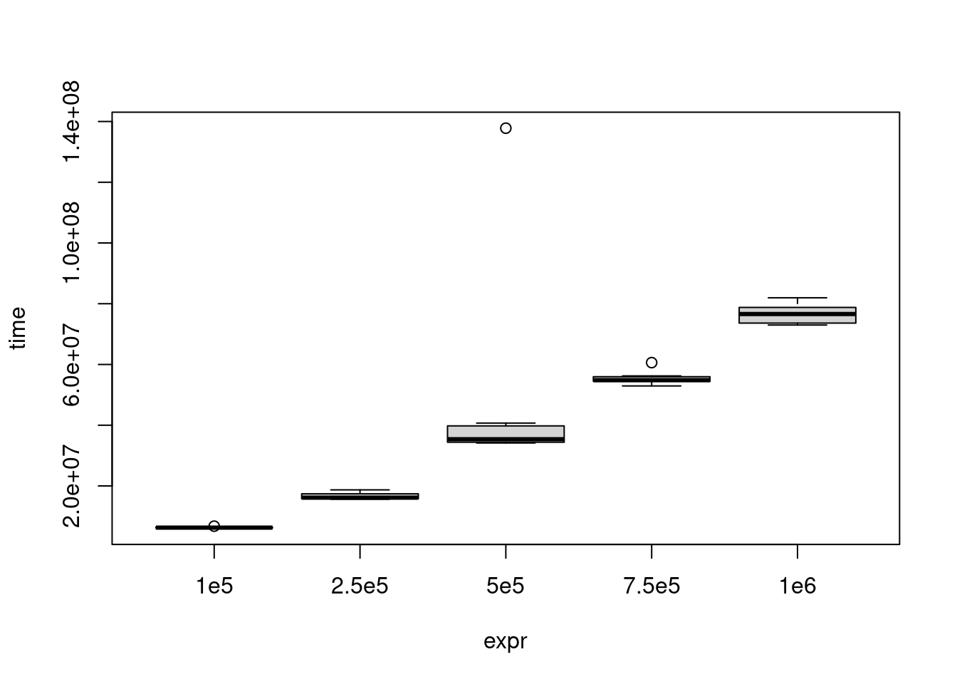
If you are processing all elements of two data sets, and one data set is bigger, then the bigger data set will take longer to process. However, it’s important to realize that how much longer it takes is not always directly proportional to how much bigger it is. That is, if you have two data sets and one is two times the size of the other, it is not guaranteed that the larger one will take twice as long to process. It could take 1.5 times longer or even four times longer. It depends on which operations are used to process the data set.
In this exercise, you’ll use the microbenchmark package, which was covered in the Writing Efficient R Code course.
Note: Numbers are specified using scientific notation
# Load the microbenchmark packagelibrary(microbenchmark)# Compare the timings for sorting different sizes of vectormb <-microbenchmark(# Sort a random normal vector length 1e5"1e5"=sort(rnorm(1e5)),# Sort a random normal vector length 2.5e5"2.5e5"=sort(rnorm(2.5e5)),# Sort a random normal vector length 5e5"5e5"=sort(rnorm(5e5)),"7.5e5"=sort(rnorm(7.5e5)),"1e6"=sort(rnorm(1e6)),times =10)# Plot the resulting benchmark objectplot(mb)
Reading a big.matrix object
In this exercise, you’ll create your first file-backed big.matrix object using the read.big.matrix() function. The function is meant to look similar to read.table() but, in addition, it needs to know what type of numeric values you want to read (“char”, “short”, “integer”, “double”), it needs the name of the file that will hold the matrix’s data (the backing file), and it needs the name of the file to hold information about the matrix (a descriptor file). The result will be a file on the disk holding the value read in along with a descriptor file which holds extra information (like the number of columns and rows) about the resulting big.matrix object.
# Load the bigmemory packagelibrary(bigmemory)# Create the big.matrix object: xx <-read.big.matrix("mortgage-sample.csv", header =TRUE, type ="integer", backingfile ="mortgage-sample.bin", descriptorfile ="mortgage-sample.desc")# Find the dimensions of xdim(x)
[1] 70000 16
Attaching a big.matrix object
Now that the big.matrix object is on the disk, we can use the information stored in the descriptor file to instantly make it available during an R session. This means that you don’t have to reimport the data set, which takes more time for larger files. You can simply point the bigmemory package at the existing structures on the disk and begin accessing data without the wait.
# Attach mortgage-sample.descmort <-attach.big.matrix("mortgage-sample.desc")# Find the dimensions of mortdim(mort)