Intermediate Python

Published

September 19, 2023

Matplotlib

Line plot (1)

With matplotlib, you can create a bunch of different plots in Python. The most basic plot is the line plot. A general recipe is given here.

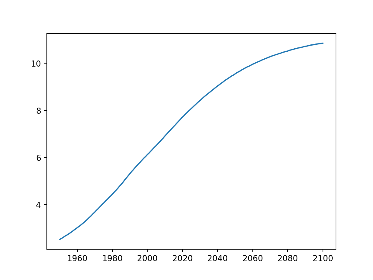
import matplotlib.pyplot as plt plt.plot(x,y) plt.show() In the video, you already saw how much the world population has grown over the past years. Will it continue to do so? The world bank has estimates of the world population for the years 1950 up to 2100. The years are loaded in your workspace as a list called year, and the corresponding populations as a list called pop.

This course touches on a lot of concepts you may have forgotten, so if you ever need a quick refresher, download the Python For Data Science Cheat Sheet and keep it handy!

# Print the last item from year and pop

year = [1950, 1951, 1952, 1953, 1954, 1955, 1956, 1957, 1958, 1959, 
        1960, 1961, 1962, 1963, 1964, 1965, 1966, 1967, 1968, 1969, 1970, 
        1971, 1972, 1973, 1974, 1975, 1976, 1977, 1978, 1979, 1980, 1981, 
        1982, 1983, 1984, 1985, 1986, 1987, 1988, 1989, 1990, 1991, 1992, 
        1993, 1994, 1995, 1996, 1997, 1998, 1999, 2000, 2001, 2002, 2003, 
        2004, 2005, 2006, 2007, 2008, 2009, 2010, 2011, 2012, 2013, 2014, 
        2015, 2016, 2017, 2018, 2019, 2020, 2021, 2022, 2023, 2024, 2025, 
        2026, 2027, 2028, 2029, 2030, 2031, 2032, 2033, 2034, 2035, 2036, 
        2037, 2038, 2039, 2040, 2041, 2042, 2043, 2044, 2045, 2046, 2047, 
        2048, 2049, 2050, 2051, 2052, 2053, 2054, 2055, 2056, 2057, 2058, 
        2059, 2060, 2061, 2062, 2063, 2064, 2065, 2066, 2067, 2068, 2069, 
        2070, 2071, 2072, 2073, 2074, 2075, 2076, 2077, 2078, 2079, 2080, 
        2081, 2082, 2083, 2084, 2085, 2086, 2087, 2088, 2089, 2090, 2091, 
        2092, 2093, 2094, 2095, 2096, 2097, 2098, 2099, 2100]

pop = [2.53, 2.57, 2.62, 2.67, 2.71, 2.76, 2.81, 2.86, 2.92, 2.97, 3.03, 
      3.08, 3.14, 3.2, 3.26, 3.33, 3.4, 3.47, 3.54, 3.62, 3.69, 3.77,
      3.84, 3.92, 4, 4.07, 4.15, 4.22, 4.3, 4.37, 4.45, 4.53, 4.61, 
      4.69, 4.78, 4.86, 4.95, 5.05, 5.14, 5.23, 5.32, 5.41, 5.49, 
      5.58, 5.66, 5.74, 5.82, 5.9, 5.98, 6.05, 6.13, 6.2, 6.28, 6.36,
      6.44, 6.51, 6.59, 6.67, 6.75, 6.83, 6.92, 7, 7.08, 7.16, 7.24, 
      7.32, 7.4, 7.48, 7.56, 7.64, 7.72, 7.79, 7.87, 7.94, 8.01, 8.08, 
      8.15, 8.22, 8.29, 8.36, 8.42, 8.49, 8.56, 8.62, 8.68, 8.74, 8.8, 
      8.86, 8.92, 8.98, 9.04, 9.09, 9.15, 9.2, 9.26, 9.31, 9.36, 9.41, 
      9.46, 9.5, 9.55, 9.6, 9.64, 9.68, 9.73, 9.77, 9.81, 9.85, 9.88, 9.92, 
      9.96, 9.99, 10.03, 10.06, 10.09, 10.13, 10.16, 10.19, 10.22, 10.25, 
      10.28, 10.31, 10.33, 10.36, 10.38, 10.41, 10.43, 10.46, 10.48, 10.5, 
      10.52, 10.55, 10.57, 10.59, 10.61, 10.63, 10.65, 10.66, 10.68, 10.7, 
      10.72, 10.73, 10.75, 10.77, 10.78, 10.79, 10.81, 10.82, 10.83, 10.84, 10.85]

print(year[-1])
2100
print(pop[-1])
10.85
# Import matplotlib.pyplot as plt
import matplotlib.pyplot as plt

# Make a line plot: year on the x-axis, pop on the y-axis

plt.plot(year, pop)
# Display the plot with plt.show()

plt.show()

Line plot (3)

Now that you’ve built your first line plot, let’s start working on the data that professor Hans Rosling used to build his beautiful bubble chart. It was collected in 2007. Two lists are available for you:

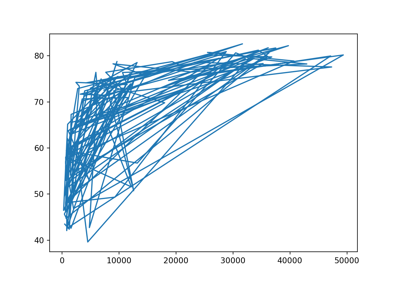
life_exp which contains the life expectancy for each country and gdp_cap, which contains the GDP per capita (i.e. per person) for each country expressed in US Dollars. GDP stands for Gross Domestic Product. It basically represents the size of the economy of a country. Divide this by the population and you get the GDP per capita.

matplotlib.pyplot is already imported as plt, so you can get started straight away.

# Print the last item of gdp_cap and life_exp

gdp_cap = [974.5803384, 5937.029526, 6223.367465, 4797.231267, 12779.37964, 
            34435.36744, 36126.4927, 29796.04834, 1391.253792, 33692.60508, 
            1441.284873, 3822.137084, 7446.298803, 12569.85177, 9065.800825, 
            10680.79282, 1217.032994, 430.0706916, 1713.778686, 2042.09524, 
            36319.23501, 706.016537, 1704.063724, 13171.63885, 4959.114854, 
            7006.580419, 986.1478792, 277.5518587, 3632.557798, 9645.06142, 
            1544.750112, 14619.22272, 8948.102923, 22833.30851, 35278.41874, 
            2082.481567, 6025.374752, 6873.262326, 5581.180998, 5728.353514, 
            12154.08975, 641.3695236, 690.8055759, 33207.0844, 30470.0167, 
            13206.48452, 752.7497265, 32170.37442, 1327.60891, 27538.41188, 
            5186.050003, 942.6542111, 579.231743, 1201.637154, 3548.330846, 
            39724.97867, 18008.94444, 36180.78919, 2452.210407, 3540.651564, 
            11605.71449, 4471.061906, 40675.99635, 25523.2771, 28569.7197, 
            7320.880262, 31656.06806, 4519.461171, 1463.249282, 1593.06548, 
            23348.13973, 47306.98978, 10461.05868, 1569.331442, 414.5073415, 
            12057.49928, 1044.770126, 759.3499101, 12451.6558, 1042.581557, 
            1803.151496, 10956.99112, 11977.57496, 3095.772271, 9253.896111, 
            3820.17523, 823.6856205, 944, 4811.060429, 1091.359778, 36797.93332, 
            25185.00911, 2749.320965, 619.6768924, 2013.977305, 49357.19017, 
            22316.19287, 2605.94758, 9809.185636, 4172.838464, 7408.905561, 
            3190.481016, 15389.92468, 20509.64777, 19328.70901, 7670.122558, 
            10808.47561, 863.0884639, 1598.435089, 21654.83194, 1712.472136, 
            9786.534714, 862.5407561, 47143.17964, 18678.31435, 25768.25759, 
            926.1410683, 9269.657808, 28821.0637, 3970.095407, 2602.394995, 
            4513.480643, 33859.74835, 37506.41907, 4184.548089, 28718.27684, 
            1107.482182, 7458.396327, 882.9699438, 18008.50924, 7092.923025, 
            8458.276384, 1056.380121, 33203.26128, 42951.65309, 10611.46299, 
            11415.80569, 2441.576404, 3025.349798, 2280.769906, 1271.211593, 
            469.7092981]


life_exp = [43.828, 76.423, 72.301, 42.731, 75.32, 81.235, 79.829, 75.635, 
             64.062, 79.441, 56.728, 65.554, 74.852, 50.728, 72.39, 73.005, 
             52.295, 49.58, 59.723, 50.43, 80.653, 44.741, 50.651, 78.553, 
             72.961, 72.889, 65.152, 46.462, 55.322, 78.782, 48.328, 75.748, 
             78.273, 76.486, 78.332, 54.791, 72.235, 74.994, 71.338, 71.878, 
             51.579, 58.04, 52.947, 79.313, 80.657, 56.735, 59.448, 79.406, 
             60.022, 79.483, 70.259, 56.007, 46.388, 60.916, 70.198, 82.208, 
             73.338, 81.757, 64.698, 70.65, 70.964, 59.545, 78.885, 80.745, 
             80.546, 72.567, 82.603, 72.535, 54.11, 67.297, 78.623, 77.588, 
             71.993, 42.592, 45.678, 73.952, 59.443, 48.303, 74.241, 54.467, 
             64.164, 72.801, 76.195, 66.803, 74.543, 71.164, 42.082, 62.069, 
             52.906, 63.785, 79.762, 80.204, 72.899, 56.867, 46.859, 80.196, 
             75.64, 65.483, 75.537, 71.752, 71.421, 71.688, 75.563, 78.098, 
             78.746, 76.442, 72.476, 46.242, 65.528, 72.777, 63.062, 74.002, 
             42.568, 79.972, 74.663, 77.926, 48.159, 49.339, 80.941, 72.396, 
             58.556, 39.613, 80.884, 81.701, 74.143, 78.4, 52.517, 70.616, 
             58.42, 69.819, 73.923, 71.777, 51.542, 79.425, 78.242, 76.384, 
             73.747, 74.249, 73.422, 62.698, 42.384, 43.487]


print(gdp_cap[-1])
469.7092981
print(life_exp[-1])
43.487
plt.plot(gdp_cap, life_exp)

# Display the plot

plt.show()

Scatter Plot (1)

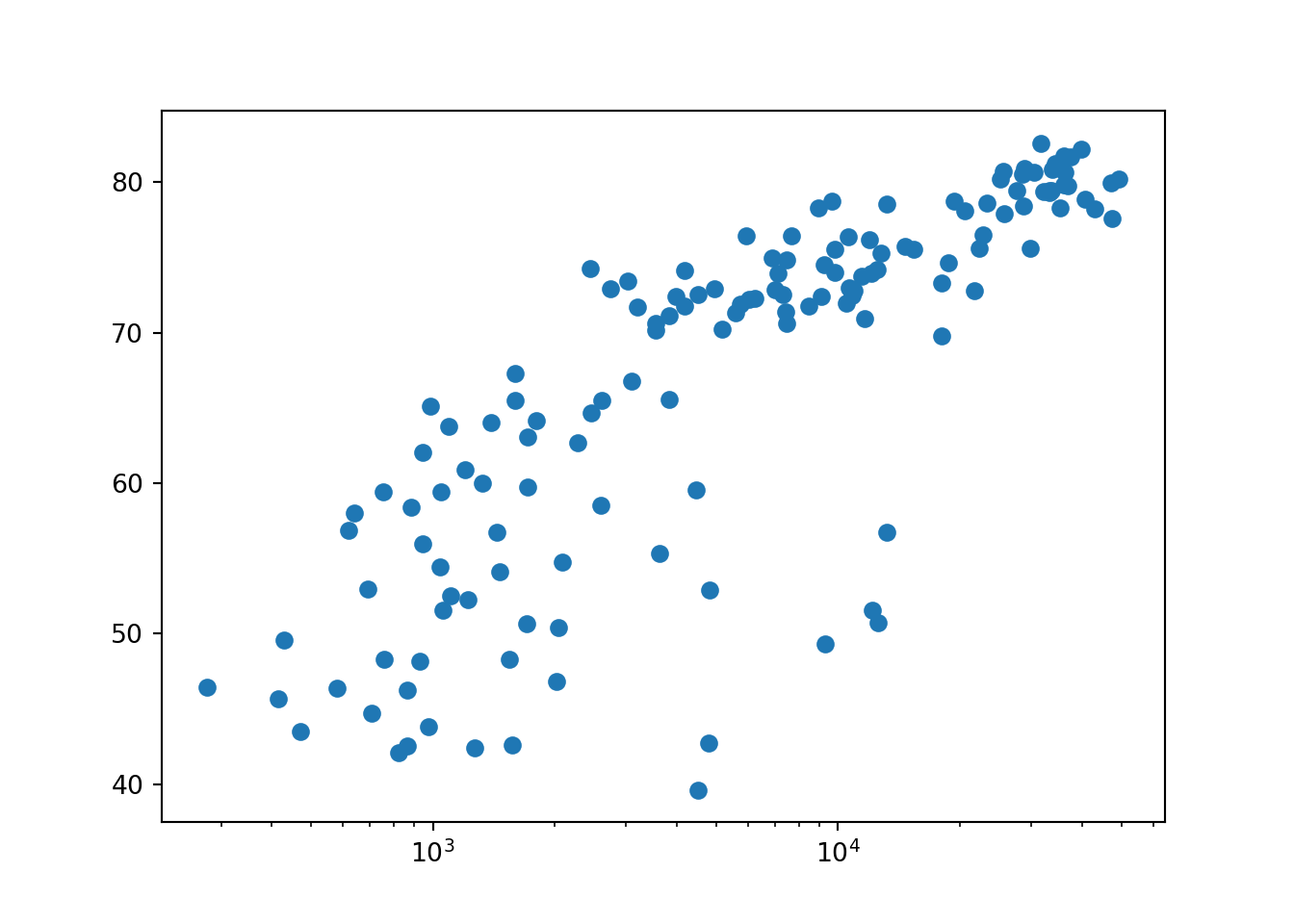
When you have a time scale along the horizontal axis, the line plot is your friend. But in many other cases, when you’re trying to assess if there’s a correlation between two variables, for example, the scatter plot is the better choice. Below is an example of how to build a scatter plot.

import matplotlib.pyplot as plt plt.scatter(x,y) plt.show() Let’s continue with the gdp_cap versus life_exp plot, the GDP and life expectancy data for different countries in 2007. Maybe a scatter plot will be a better alternative?

# Change the line plot below to a scatter plot
plt.scatter(gdp_cap, life_exp)

# Put the x-axis on a logarithmic scale
plt.xscale('log')
# Show plot.
plt.show()

Scatter plot (2)

In the previous exercise, you saw that the higher GDP usually corresponds to a higher life expectancy. In other words, there is a positive correlation.

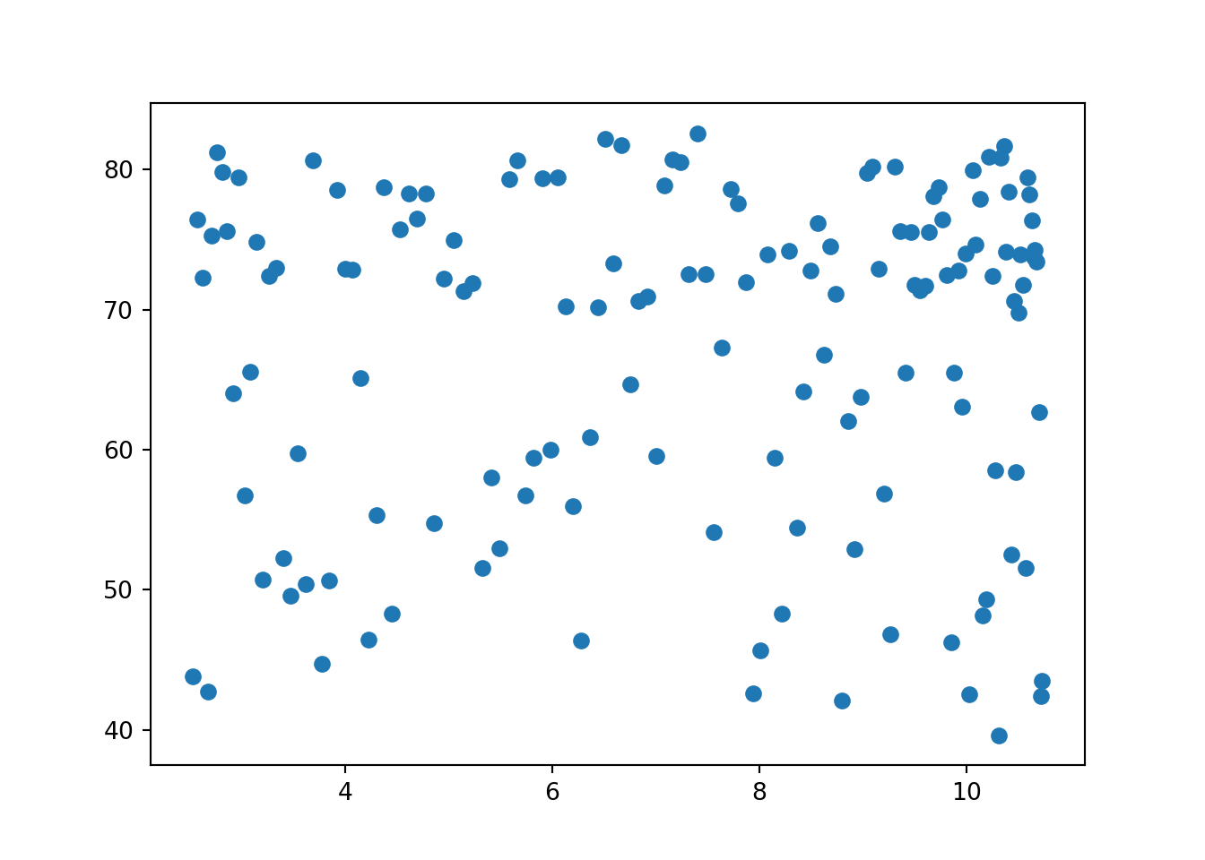
Do you think there’s a relationship between population and life expectancy of a country? The list life_exp from the previous exercise is already available. In addition, now also pop is available, listing the corresponding populations for the countries in 2007. The populations are in millions of people.

# Build Scatter plot
pop = pop[0:142]
plt.scatter(pop[0:142], life_exp)

# Show plot
plt.show()

Build a histogram (1)

life_exp, the list containing data on the life expectancy for different countries in 2007, is available in your Python shell.

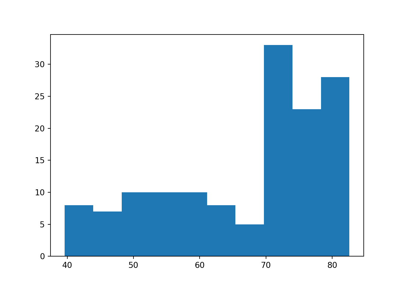
To see how life expectancy in different countries is distributed, let’s create a histogram of life_exp.

matplotlib.pyplot is already available as plt.

# Create histogram of life_exp data
plt.hist(life_exp)

# Display histogram
plt.show()

Build a histogram (2): bins

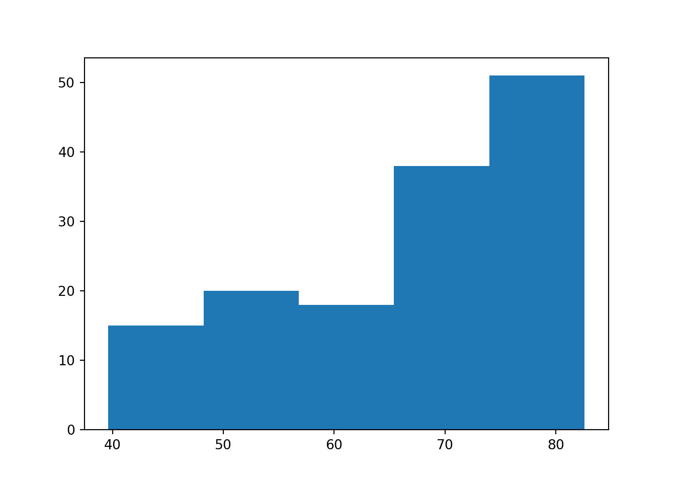
In the previous exercise, you didn’t specify the number of bins. By default, Python sets the number of bins to 10 in that case. The number of bins is pretty important. Too few bins will oversimplify reality and won’t show you the details. Too many bins will overcomplicate reality and won’t show the bigger picture.

To control the number of bins to divide your data in, you can set the bins argument.

That’s exactly what you’ll do in this exercise. You’ll be making two plots here. The code in the script already includes plt.show() and plt.clf() calls; plt.show() displays a plot; plt.clf() cleans it up again so you can start afresh.

As before, life_exp is available and matplotlib.pyplot is imported as plt.

# Build histogram with 5 bins
plt.hist(life_exp, bins= 5)

# Show and clean up plot
plt.show()

plt.clf()

# Build histogram with 20 bins

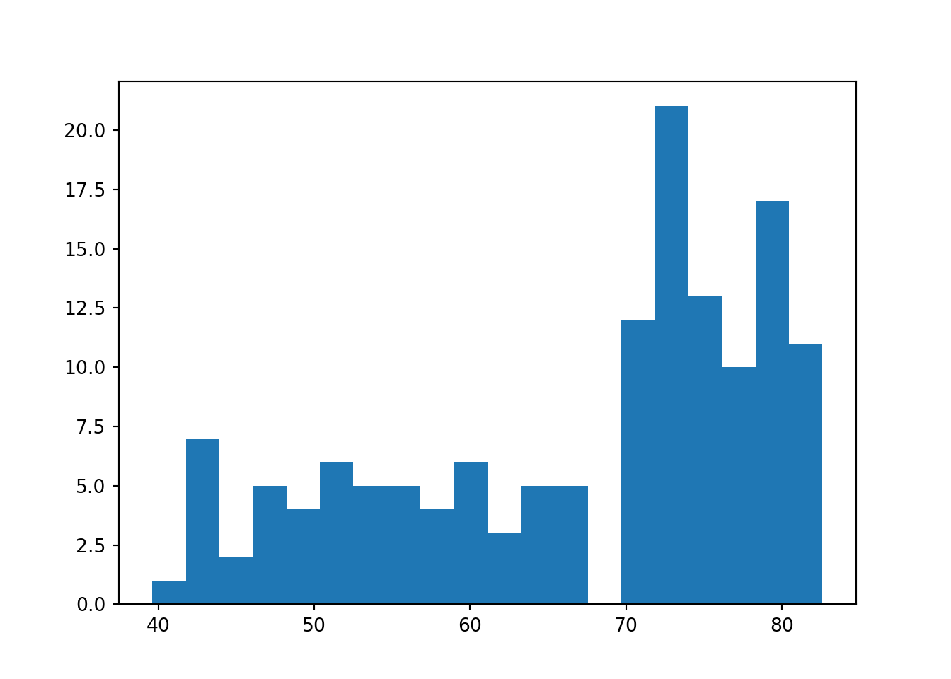
plt.hist(life_exp, bins= 20)

# Show and clean up again
plt.show()

#plt.clf()

Build a histogram (3): compare

In the video, you saw population pyramids for the present day and for the future. Because we were using a histogram, it was very easy to make a comparison.

Let’s do a similar comparison. life_exp contains life expectancy data for different countries in 2007. You also have access to a second list now, life_exp1950, containing similar data for 1950. Can you make a histogram for both datasets?

You’ll again be making two plots. The plt.show() and plt.clf() commands to render everything nicely are already included. Also matplotlib.pyplot is imported for you, as plt.

# Histogram of life_exp, 15 bins

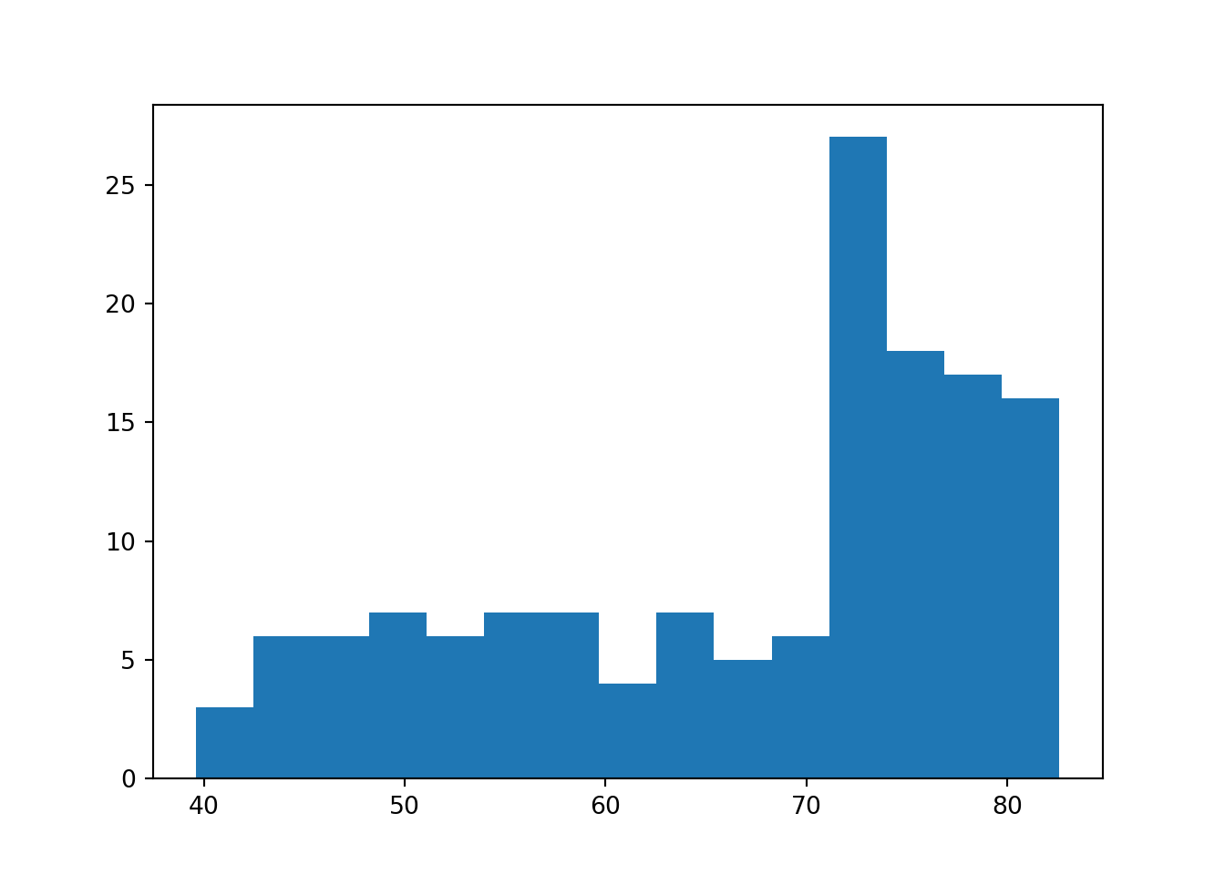
plt.hist(life_exp, bins = 15)
# Show and clear plot
plt.show()

plt.clf()

# Histogram of life_exp1950, 15 bins
life_exp1950 = [28.8, 55.23, 43.08, 30.02, 62.48, 69.12, 66.8, 50.94, 37.48, 
                 68, 38.22, 40.41, 53.82, 47.62, 50.92, 59.6, 31.98, 39.03, 39.42, 
                 38.52, 68.75, 35.46, 38.09, 54.74, 44, 50.64, 40.72, 39.14, 42.11, 
                 57.21, 40.48, 61.21, 59.42, 66.87, 70.78, 34.81, 45.93, 48.36, 
                 41.89, 45.26, 34.48, 35.93, 34.08, 66.55, 67.41, 37, 30, 67.5, 
                 43.15, 65.86, 42.02, 33.61, 32.5, 37.58, 41.91, 60.96, 64.03, 
                 72.49, 37.37, 37.47, 44.87, 45.32, 66.91, 65.39, 65.94, 58.53, 
                 63.03, 43.16, 42.27, 50.06, 47.45, 55.56, 55.93, 42.14, 38.48, 
                 42.72, 36.68, 36.26, 48.46, 33.68, 40.54, 50.99, 50.79, 42.24, 
                 59.16, 42.87, 31.29, 36.32, 41.72, 36.16, 72.13, 69.39, 42.31, 
                 37.44, 36.32, 72.67, 37.58, 43.44, 55.19, 62.65, 43.9, 47.75, 
                 61.31, 59.82, 64.28, 52.72, 61.05, 40, 46.47, 39.88, 37.28, 58, 
                 30.33, 60.4, 64.36, 65.57, 32.98, 45.01, 64.94, 57.59, 38.64, 
                 41.41, 71.86, 69.62, 45.88, 58.5, 41.22, 50.85, 38.6, 59.1, 44.6, 
                 43.58, 39.98, 69.18, 68.44, 66.07, 55.09, 40.41, 43.16, 32.55, 
                 42.04, 48.45]
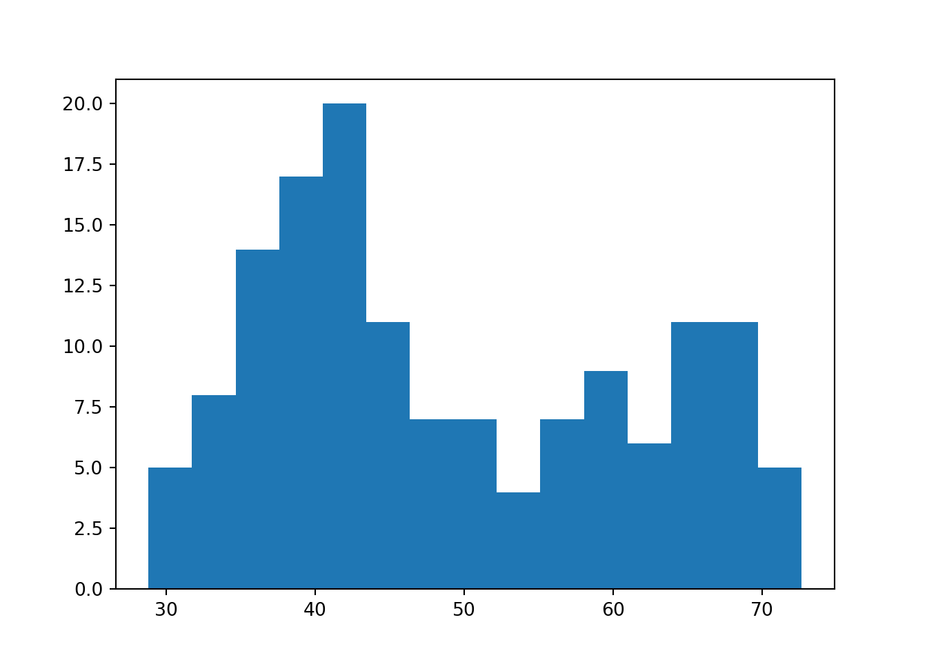
plt.hist(life_exp1950, bins = 15)
# Show and clear plot again
plt.show()

#plt.clf()

Labels

It’s time to customize your own plot. This is the fun part, you will see your plot come to life!

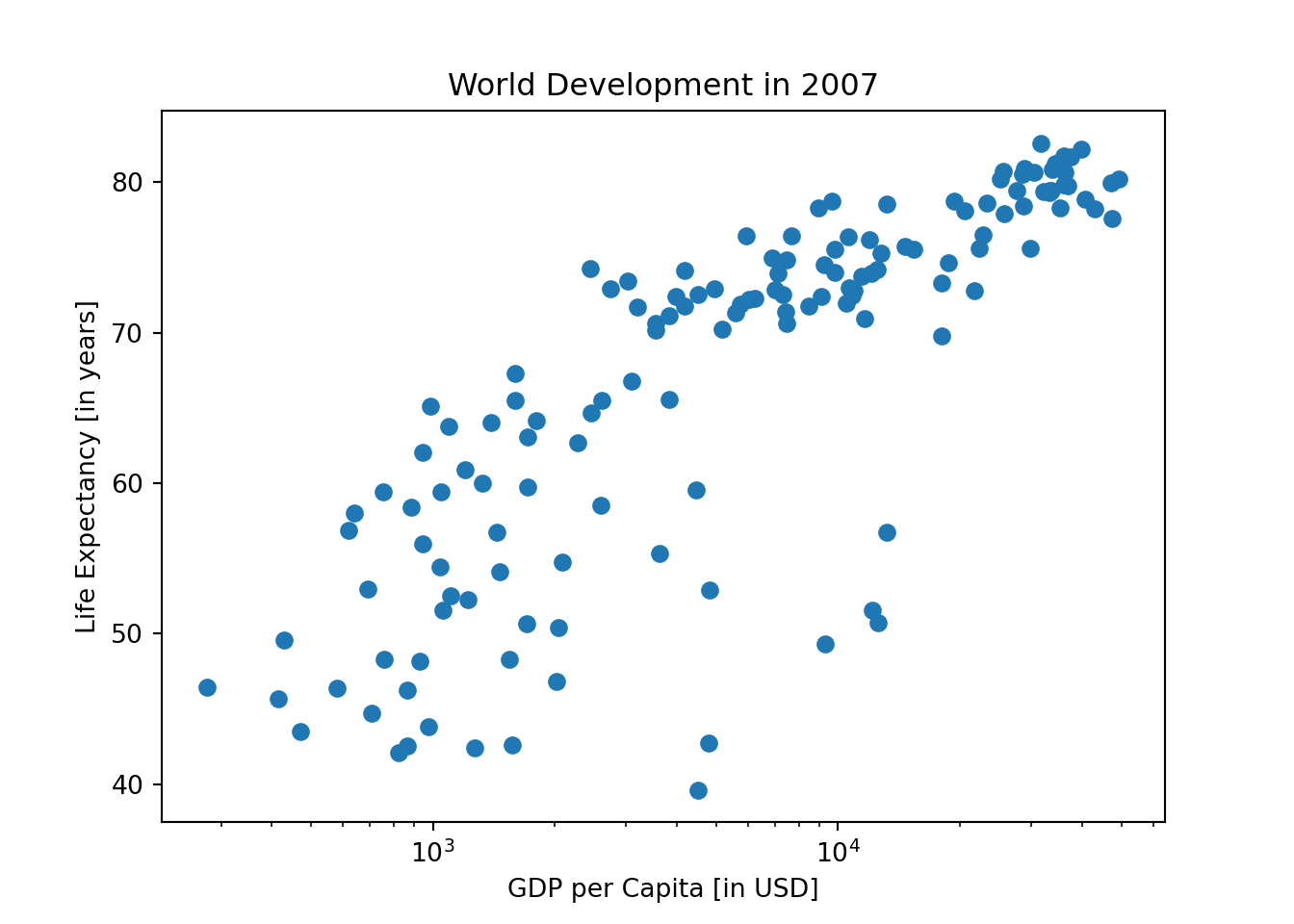
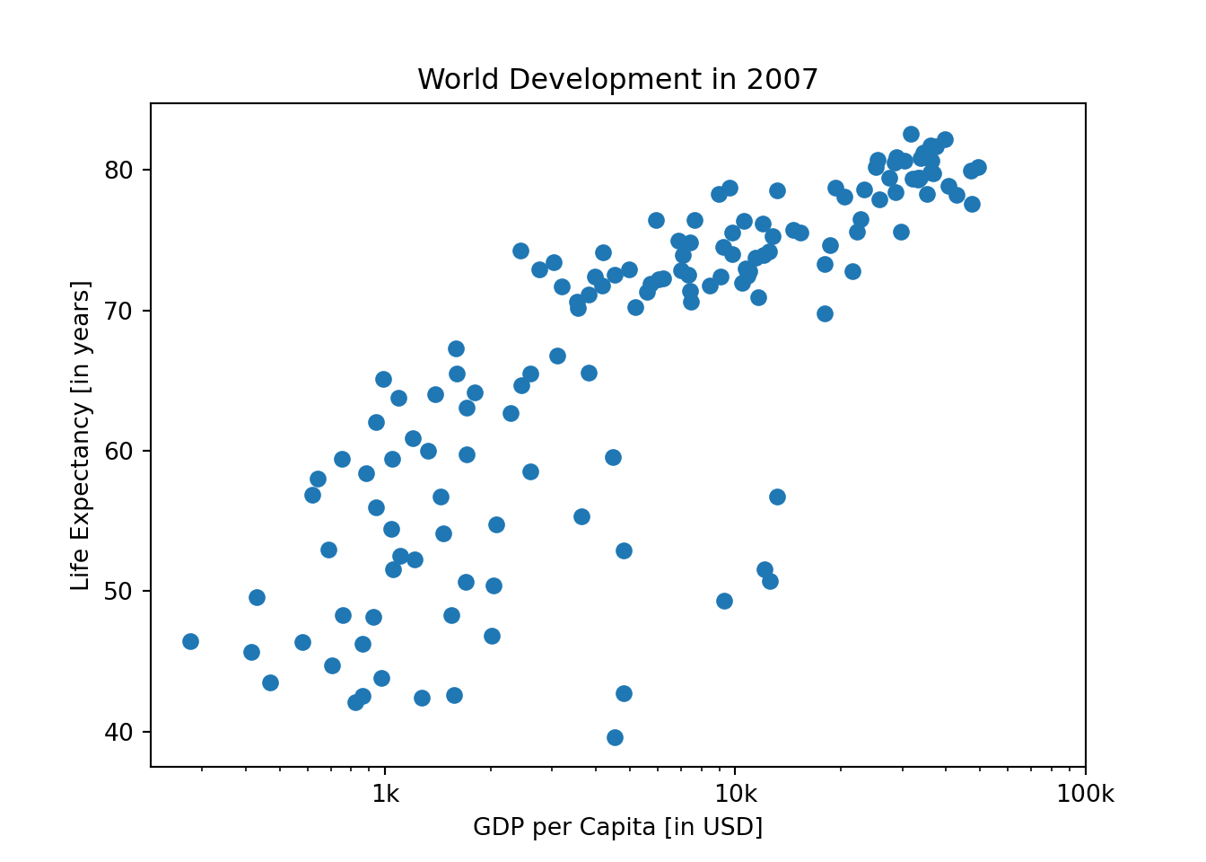
You’re going to work on the scatter plot with world development data: GDP per capita on the x-axis (logarithmic scale), life expectancy on the y-axis. The code for this plot is available in the script.

As a first step, let’s add axis labels and a title to the plot. You can do this with the xlabel(), ylabel() and title() functions, available in matplotlib.pyplot. This sub-package is already imported as plt.

# Basic scatter plot, log scale
plt.scatter(gdp_cap, life_exp)
plt.xscale('log') 

# Strings
xlab = 'GDP per Capita [in USD]'
ylab = 'Life Expectancy [in years]'
title = 'World Development in 2007'

# Add axis labels
plt.xlabel(xlab)
plt.ylabel(ylab)


# Add title
plt.title(title)

# After customizing, display the plot
plt.show()

Ticks

The customizations you’ve coded up to now are available in the script, in a more concise form.

In the video, Hugo has demonstrated how you could control the y-ticks by specifying two arguments:

plt.yticks([0,1,2], [“one”,“two”,“three”]) In this example, the ticks corresponding to the numbers 0, 1 and 2 will be replaced by one, two and three, respectively.

Let’s do a similar thing for the x-axis of your world development chart, with the xticks() function. The tick values 1000, 10000 and 100000 should be replaced by 1k, 10k and 100k. To this end, two lists have already been created for you: tick_val and tick_lab.

# Scatter plot
plt.scatter(gdp_cap, life_exp)

# Previous customizations
plt.xscale('log') 
plt.xlabel('GDP per Capita [in USD]')
plt.ylabel('Life Expectancy [in years]')
plt.title('World Development in 2007')

# Definition of tick_val and tick_lab
tick_val = [1000, 10000, 100000]
tick_lab = ['1k', '10k', '100k']

# Adapt the ticks on the x-axis
plt.xticks(tick_val, tick_lab)
([<matplotlib.axis.XTick object at 0x7f21a695e150>, <matplotlib.axis.XTick object at 0x7f21a81f2810>, <matplotlib.axis.XTick object at 0x7f21abb9db90>], [Text(1000, 0, '1k'), Text(10000, 0, '10k'), Text(100000, 0, '100k')])
# After customizing, display the plot
plt.show()

Sizes

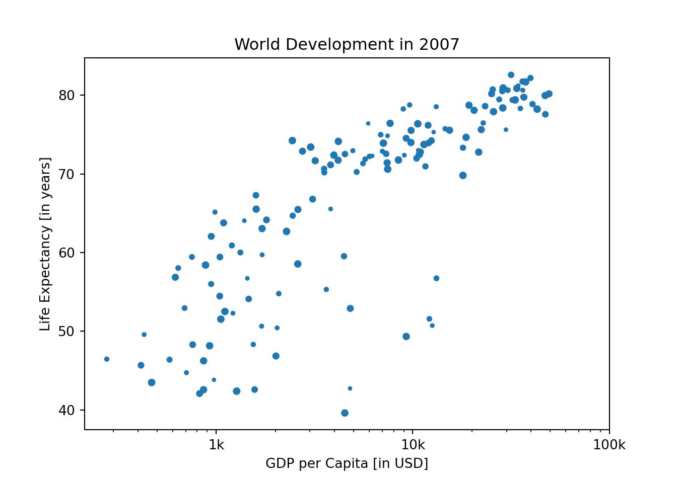
Right now, the scatter plot is just a cloud of blue dots, indistinguishable from each other. Let’s change this. Wouldn’t it be nice if the size of the dots corresponds to the population?

To accomplish this, there is a list pop loaded in your workspace. It contains population numbers for each country expressed in millions. You can see that this list is added to the scatter method, as the argument s, for size.

 # Import numpy as np

import numpy as np
# Store pop as a numpy array: np_pop
np_pop = np.array(pop)

# Double np_pop

np_pop = np_pop*2
# Update: set s argument to np_pop
plt.scatter(gdp_cap, life_exp,  s = np_pop)

# Previous customizations
plt.xscale('log') 
plt.xlabel('GDP per Capita [in USD]')
plt.ylabel('Life Expectancy [in years]')
plt.title('World Development in 2007')
plt.xticks([1000, 10000, 100000],['1k', '10k', '100k'])
([<matplotlib.axis.XTick object at 0x7f21a8180e90>, <matplotlib.axis.XTick object at 0x7f21abb42810>, <matplotlib.axis.XTick object at 0x7f21a6922810>], [Text(1000, 0, '1k'), Text(10000, 0, '10k'), Text(100000, 0, '100k')])
# Display the plot
plt.show()

Colors

The code you’ve written up to now is available in the script.

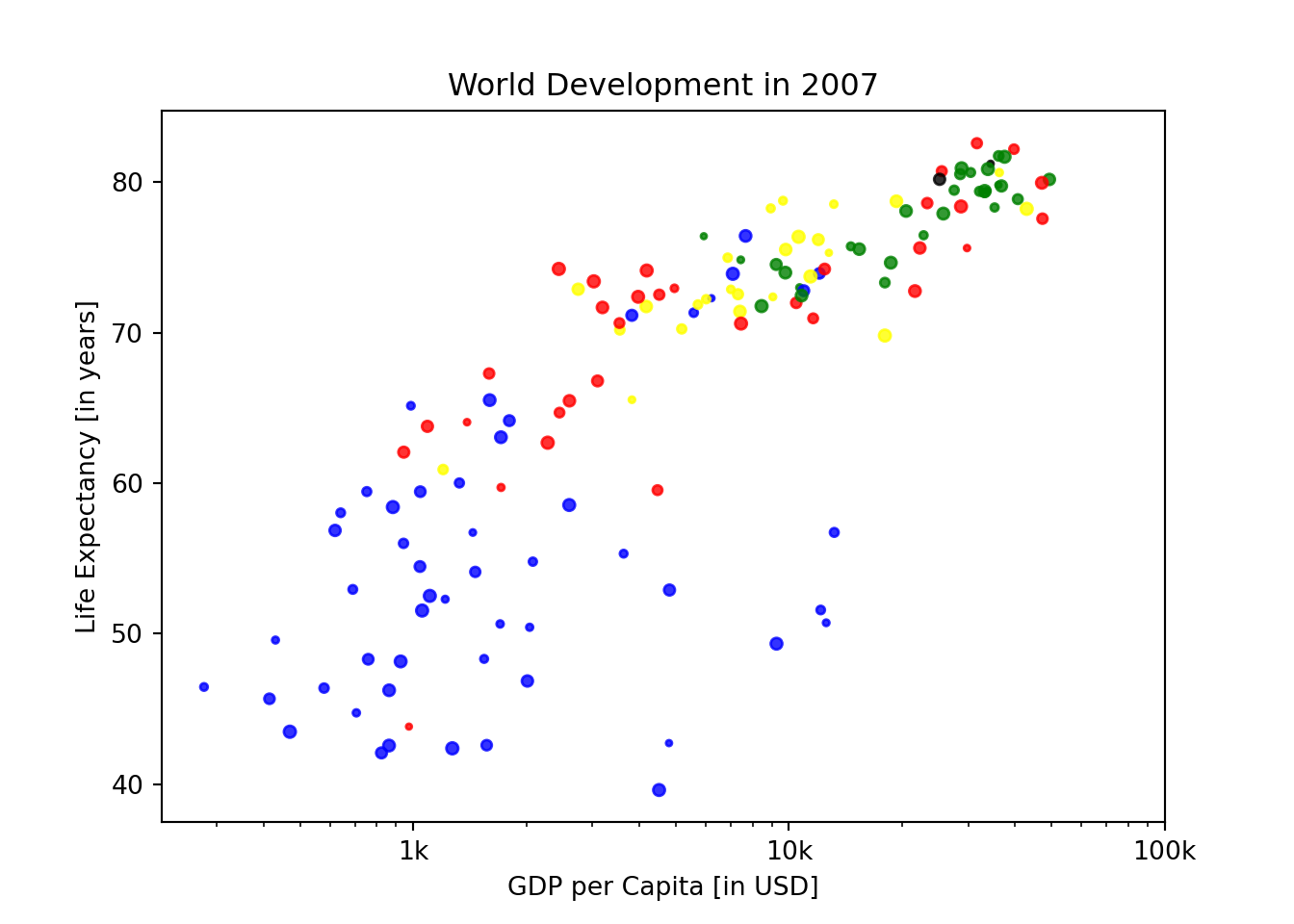
The next step is making the plot more colorful! To do this, a list col has been created for you. It’s a list with a color for each corresponding country, depending on the continent the country is part of.

How did we make the list col you ask? The Gapminder data contains a list continent with the continent each country belongs to. A dictionary is constructed that maps continents onto colors:

dict = { ‘Asia’:‘red’, ‘Europe’:‘green’, ‘Africa’:‘blue’, ‘Americas’:‘yellow’, ‘Oceania’:‘black’ } Nothing to worry about now; you will learn about dictionaries in the next chapter.

# Specify c and alpha inside plt.scatter()
col =  ["red", "green", "blue", "blue", "yellow", "black", "green", 
        "red", "red", "green", "blue", "yellow", "green", "blue", "yellow", 
        "green", "blue", "blue", "red", "blue", "yellow", "blue", "blue", 
        "yellow", "red", "yellow", "blue", "blue", "blue", "yellow", 
        "blue", "green", "yellow", "green", "green", "blue", "yellow", 
        "yellow", "blue", "yellow", "blue", "blue", "blue", "green", 
        "green", "blue", "blue", "green", "blue", "green", "yellow", 
        "blue", "blue", "yellow", "yellow", "red", "green", "green", 
        "red", "red", "red", "red", "green", "red", "green", "yellow", 
        "red", "red", "blue", "red", "red", "red", "red", "blue", "blue", 
        "blue", "blue", "blue", "red", "blue", "blue", "blue", "yellow", 
        "red", "green", "blue", "blue", "red", "blue", "red", "green", 
        "black", "yellow", "blue", "blue", "green", "red", "red", "yellow", 
        "yellow", "yellow", "red", "green", "green", "yellow", "blue", 
        "green", "blue", "blue", "red", "blue", "green", "blue", "red", 
        "green", "green", "blue", "blue", "green", "red", "blue", "blue", 
        "green", "green", "red", "red", "blue", "red", "blue", "yellow", 
        "blue", "green", "blue", "green", "yellow", "yellow", "yellow", 
        "red", "red", "red", "blue", "blue"]
plt.scatter(x = gdp_cap, y = life_exp, s = np.array(pop) * 2, alpha = 0.8, c = col)

# Previous customizations
plt.xscale('log') 
plt.xlabel('GDP per Capita [in USD]')
plt.ylabel('Life Expectancy [in years]')
plt.title('World Development in 2007')
plt.xticks([1000,10000,100000], ['1k','10k','100k'])
([<matplotlib.axis.XTick object at 0x7f21a69598d0>, <matplotlib.axis.XTick object at 0x7f21a6390f50>, <matplotlib.axis.XTick object at 0x7f21a6312810>], [Text(1000, 0, '1k'), Text(10000, 0, '10k'), Text(100000, 0, '100k')])
# Show the plot
plt.show()

Additional Customizations

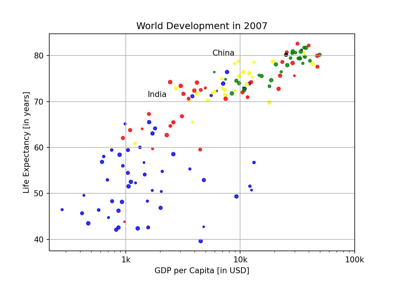
If you have another look at the script, under # Additional Customizations, you’ll see that there are two plt.text() functions now. They add the words “India” and “China” in the plot.

# Scatter plot
plt.scatter(x = gdp_cap, y = life_exp, s = np.array(pop) * 2, c = col, alpha = 0.8)

# Previous customizations
plt.xscale('log') 
plt.xlabel('GDP per Capita [in USD]')
plt.ylabel('Life Expectancy [in years]')
plt.title('World Development in 2007')
plt.xticks([1000,10000,100000], ['1k','10k','100k'])
([<matplotlib.axis.XTick object at 0x7f21a6912590>, <matplotlib.axis.XTick object at 0x7f21a63bd510>, <matplotlib.axis.XTick object at 0x7f21a622db90>], [Text(1000, 0, '1k'), Text(10000, 0, '10k'), Text(100000, 0, '100k')])
# Additional customizations
plt.text(1550, 71, 'India')
plt.text(5700, 80, 'China')

# Add grid() call

plt.grid(True)
# Show the plot
plt.show()

Dictionaries & Pandas

Motivation for dictionaries

To see why dictionaries are useful, have a look at the two lists defined in the script. countries contains the names of some European countries. capitals lists the corresponding names of their capital.

# Definition of countries and capital
countries = ['spain', 'france', 'germany', 'norway']
capitals = ['madrid', 'paris', 'berlin', 'oslo']

# Get index of 'germany': ind_ger
ind_ger = countries.index("germany")

# Use ind_ger to print out capital of Germany
print(capitals[ind_ger])
berlin

Create dictionary

The countries and capitals lists are again available in the script. It’s your job to convert this data to a dictionary where the country names are the keys and the capitals are the corresponding values. As a refresher, here is a recipe for creating a dictionary:

my_dict = {
   "key1":"value1",
   "key2":"value2",
}

In this recipe, both the keys and the values are strings. This will also be the case for this exercise.

# Definition of countries and capital
countries = ['spain', 'france', 'germany', 'norway']
capitals = ['madrid', 'paris', 'berlin', 'oslo']

# From string in countries and capitals, create dictionary europe
europe = { 'spain':'madrid', 'france': 'paris','germany' : 'berlin', 'norway' : 'oslo'}

# Print europe
print(europe)
{'spain': 'madrid', 'france': 'paris', 'germany': 'berlin', 'norway': 'oslo'}

Access dictionary

If the keys of a dictionary are chosen wisely, accessing the values in a dictionary is easy and intuitive. For example, to get the capital for France from europe you can use:

europe[‘france’] Here, ‘france’ is the key and ‘paris’ the value is returned.

# Definition of dictionary
europe = {'spain':'madrid', 'france':'paris', 'germany':'berlin', 'norway':'oslo' }

# Print out the keys in europe
print(europe.keys())
dict_keys(['spain', 'france', 'germany', 'norway'])
# Print out value that belongs to key 'norway'

print(europe['norway'])
oslo

Dictionary Manipulation (1)

If you know how to access a dictionary, you can also assign a new value to it. To add a new key-value pair to europe you can use something like this:

# Definition of dictionary
europe = {'spain':'madrid', 'france':'paris', 'germany':'berlin', 'norway':'oslo' }

# Add italy to europe

europe['italy'] = 'rome'
# Print out italy in europe

print('italy' in europe)
True
# Add poland to europe

europe['poland'] = 'warsaw'
# Print europe
print(europe)
{'spain': 'madrid', 'france': 'paris', 'germany': 'berlin', 'norway': 'oslo', 'italy': 'rome', 'poland': 'warsaw'}

Dictionary Manipulation (2)

Somebody thought it would be funny to mess with your accurately generated dictionary. An adapted version of the europe dictionary is available in the script.

Can you clean up? Do not do this by adapting the definition of europe, but by adding Python commands to the script to update and remove key:value pairs.

# Definition of dictionary
europe = {'spain':'madrid', 'france':'paris', 'germany':'bonn',
          'norway':'oslo', 'italy':'rome', 'poland':'warsaw',
          'australia':'vienna' }

# Update capital of germany

europe['germany'] = 'berlin'
# Remove australia

del(europe['australia'])
# Print europe
print(europe)
{'spain': 'madrid', 'france': 'paris', 'germany': 'berlin', 'norway': 'oslo', 'italy': 'rome', 'poland': 'warsaw'}

Dictionariception

Remember lists? They could contain anything, even other lists. Well, for dictionaries the same holds. Dictionaries can contain key:value pairs where the values are again dictionaries.

As an example, have a look at the script where another version of europe - the dictionary you’ve been working with all along - is coded. The keys are still the country names, but the values are dictionaries that contain more information than just the capital.

It’s perfectly possible to chain square brackets to select elements. To fetch the population for Spain from europe, for example, you need:

# Dictionary of dictionaries
europe = { 'spain': { 'capital':'madrid', 'population':46.77 },
           'france': { 'capital':'paris', 'population':66.03 },
           'germany': { 'capital':'berlin', 'population':80.62 },
           'norway': { 'capital':'oslo', 'population':5.084 } }


# Print out the capital of France

print(europe['spain']['capital'])
madrid
# Create sub-dictionary data
data = {'capital' : 'rome', 'population' : 59.83}

# Add data to europe under key 'italy'
europe['italy'] = data

# Print europe

print(europe)
{'spain': {'capital': 'madrid', 'population': 46.77}, 'france': {'capital': 'paris', 'population': 66.03}, 'germany': {'capital': 'berlin', 'population': 80.62}, 'norway': {'capital': 'oslo', 'population': 5.084}, 'italy': {'capital': 'rome', 'population': 59.83}}

Dictionary to DataFrame (1)

Pandas is an open source library, providing high-performance, easy-to-use data structures and data analysis tools for Python. Sounds promising!

The DataFrame is one of Pandas’ most important data structures. It’s basically a way to store tabular data where you can label the rows and the columns. One way to build a DataFrame is from a dictionary.

In the exercises that follow you will be working with vehicle data from different countries. Each observation corresponds to a country and the columns give information about the number of vehicles per capita, whether people drive left or right, and so on.

Three lists are defined in the script:

names, containing the country names for which data is available. dr, a list with booleans that tells whether people drive left or right in the corresponding country. cpc, the number of motor vehicles per 1000 people in the corresponding country. Each dictionary key is a column label and each value is a list which contains the column elements.

# Pre-defined lists
names = ['United States', 'Australia', 'Japan', 'India', 'Russia', 'Morocco', 'Egypt']
dr =  [True, False, False, False, True, True, True]
cpc = [809, 731, 588, 18, 200, 70, 45]

# Import pandas as pd

import pandas as pd
# Create dictionary my_dict with three key:value pairs: my_dict

my_dict = {'country' :names, 'drives_right' : dr, 'cars_per_cap' : cpc }
# Build a DataFrame cars from my_dict: cars
cars = pd.DataFrame(my_dict)


from IPython.display import HTML
HTML(cars.to_html())
country drives_right cars_per_cap
0 United States True 809
1 Australia False 731
2 Japan False 588
3 India False 18
4 Russia True 200
5 Morocco True 70
6 Egypt True 45

Dictionary to DataFrame (2)

The Python code that solves the previous exercise is included in the script. Have you noticed that the row labels (i.e. the labels for the different observations) were automatically set to integers from 0 up to 6?

To solve this a list row_labels has been created. You can use it to specify the row labels of the cars DataFrame. You do this by setting the index attribute of cars, that you can access as cars.index.

# Build cars DataFrame
names = ['United States', 'Australia', 'Japan', 'India', 'Russia', 'Morocco', 'Egypt']
dr =  [True, False, False, False, True, True, True]
cpc = [809, 731, 588, 18, 200, 70, 45]
cars_dict = { 'country':names, 'drives_right':dr, 'cars_per_cap':cpc }
cars = pd.DataFrame(cars_dict)
print(cars)
         country  drives_right  cars_per_cap
0  United States          True           809
1      Australia         False           731
2          Japan         False           588
3          India         False            18
4         Russia          True           200
5        Morocco          True            70
6          Egypt          True            45
# Definition of row_labels
row_labels = ['US', 'AUS', 'JPN', 'IN', 'RU', 'MOR', 'EG']

# Specify row labels of cars
cars.index = row_labels

# Print cars again
HTML(cars.to_html())
country drives_right cars_per_cap
US United States True 809
AUS Australia False 731
JPN Japan False 588
IN India False 18
RU Russia True 200
MOR Morocco True 70
EG Egypt True 45

CSV to DataFrame (1)

Putting data in a dictionary and then building a DataFrame works, but it’s not very efficient. What if you’re dealing with millions of observations? In those cases, the data is typically available as files with a regular structure. One of those file types is the CSV file, which is short for “comma-separated values”.

To import CSV data into Python as a Pandas DataFrame you can use read_csv().

Let’s explore this function with the same cars data from the previous exercises. This time, however, the data is available in a CSV file, named cars.csv. It is available in your current working directory, so the path to the file is simply ‘cars.csv’.

# Import the cars.csv data: cars

cars = pd.read_csv('data/cars.csv')
# Print out cars
HTML(cars.to_html())
Unnamed: 0 cars_per_cap country drives_right
0 US 809 United States True
1 AUS 731 Australia False
2 JAP 588 Japan False
3 IN 18 India False
4 RU 200 Russia True
5 MOR 70 Morocco True
6 EG 45 Egypt True

CSV to DataFrame (2)

Your read_csv() call to import the CSV data didn’t generate an error, but the output is not entirely what we wanted. The row labels were imported as another column without a name.

Remember index_col, an argument of read_csv(), that you can use to specify which column in the CSV file should be used as a row label? Well, that’s exactly what you need here!

Python code that solves the previous exercise is already included; can you make the appropriate changes to fix the data import?

# Fix import by including index_col
cars = pd.read_csv('data/cars.csv', index_col = 0)

# Print out cars
HTML(cars.to_html())
cars_per_cap country drives_right
US 809 United States True
AUS 731 Australia False
JAP 588 Japan False
IN 18 India False
RU 200 Russia True
MOR 70 Morocco True
EG 45 Egypt True

Square Brackets (1)

In the video, you saw that you can index and select Pandas DataFrames in many different ways. The simplest, but not the most powerful way, is to use square brackets.

In the sample code, the same cars data is imported from a CSV files as a Pandas DataFrame. To select only the cars_per_cap column from cars, you can use:

cars[‘cars_per_cap’] cars[[‘cars_per_cap’]] The single bracket version gives a Pandas Series, the double bracket version gives a Pandas DataFrame.

# Print out country column as Pandas Series

print(cars['country'])
US     United States
AUS        Australia
JAP            Japan
IN             India
RU            Russia
MOR          Morocco
EG             Egypt
Name: country, dtype: object
# Print out country column as Pandas DataFrame
print(cars[['country']])
           country
US   United States
AUS      Australia
JAP          Japan
IN           India
RU          Russia
MOR        Morocco
EG           Egypt
# Print out DataFrame with country and drives_right columns
print(cars[['country', 'drives_right']])
           country  drives_right
US   United States          True
AUS      Australia         False
JAP          Japan         False
IN           India         False
RU          Russia          True
MOR        Morocco          True
EG           Egypt          True

Square Brackets (2)

Square brackets can do more than just selecting columns. You can also use them to get rows, or observations, from a DataFrame. The following call selects the first five rows from the cars DataFrame:

cars[0:5] The result is another DataFrame containing only the rows you specified.

Pay attention: You can only select rows using square brackets if you specify a slice, like 0:4. Also, you’re using the integer indexes of the rows here, not the row labels!

# Print out first 3 observations
print(cars[0:3])
     cars_per_cap        country  drives_right
US            809  United States          True
AUS           731      Australia         False
JAP           588          Japan         False
# Print out fourth, fifth and sixth observation
print(cars[3:6])
     cars_per_cap  country  drives_right
IN             18    India         False
RU            200   Russia          True
MOR            70  Morocco          True

loc and iloc (1)

With loc and iloc you can do practically any data selection operation on DataFrames you can think of. loc is label-based, which means that you have to specify rows and columns based on their row and column labels. iloc is integer index based, so you have to specify rows and columns by their integer index like you did in the previous exercise.

Try out the following commands in the IPython Shell to experiment with loc and iloc to select observations. Each pair of commands here gives the same result.

cars.loc[‘RU’] cars.iloc[4]

cars.loc[[‘RU’]] cars.iloc[[4]]

cars.loc[[‘RU’, ‘AUS’]] cars.iloc[[4, 1]] As before, code is included that imports the cars data as a Pandas DataFrame.

# Print out observation for Japan
print(cars.loc['JAP'])
cars_per_cap      588
country         Japan
drives_right    False
Name: JAP, dtype: object
# Print out observations for Australia and Egypt
print(cars.loc[['AUS', 'EG']])
     cars_per_cap    country  drives_right
AUS           731  Australia         False
EG             45      Egypt          True

loc and iloc (2)

loc and iloc also allow you to select both rows and columns from a DataFrame. To experiment, try out the following commands in the IPython Shell. Again, paired commands produce the same result.

# Print out drives_right value of Morocco
print(cars.loc[['MOR'], 'drives_right'])
MOR    True
Name: drives_right, dtype: bool
# Print sub-DataFrame
print(cars.loc[['RU','MOR'], ['country','drives_right']])
     country  drives_right
RU    Russia          True
MOR  Morocco          True

loc and iloc (3)

It’s also possible to select only columns with loc and iloc. In both cases, you simply put a slice going from beginning to end in front of the comma:

# Print out drives_right column as Series
print(cars.loc[:, 'drives_right'])
US      True
AUS    False
JAP    False
IN     False
RU      True
MOR     True
EG      True
Name: drives_right, dtype: bool
# Print out drives_right column as DataFrame

print(cars.loc[:, ['drives_right']])
     drives_right
US           True
AUS         False
JAP         False
IN          False
RU           True
MOR          True
EG           True
# Print out cars_per_cap and drives_right as DataFrame

print(cars.loc[:, ['cars_per_cap','drives_right']])
     cars_per_cap  drives_right
US            809          True
AUS           731         False
JAP           588         False
IN             18         False
RU            200          True
MOR            70          True
EG             45          True

Logic, Control Flow and Filtering

Equality

To check if two Python values, or variables, are equal you can use ==. To check for inequality, you need !=. As a refresher, have a look at the following examples that all result in True. Feel free to try them out in the IPython Shell.

2 == (1 + 1) “intermediate” != “python” True != False “Python” != “python” When you write these comparisons in a script, you will need to wrap a print() function around them to see the output.

# Comparison of booleans
print(True == False)
False
# Comparison of integers
print(-5*15 != 75)
True
# Comparison of strings
print("pyscript" == "PyScript")
False
# Compare a boolean with an integer
print(True == 1)
True

Greater and less than

In the video, Hugo also talked about the less than and greater than signs, < and > in Python. You can combine them with an equals sign: <= and >=. Pay attention: <= is valid syntax, but =< is not.

All Python expressions in the following code chunk evaluate to True:

# Comparison of integers
x = -3 * 6
print(x >= -10)
False
# Comparison of strings
y="test"
print("test" <= y)
True
# Comparison of booleans
print(True > False)
True

Compare arrays

Out of the box, you can also use comparison operators with NumPy arrays.

Remember areas, the list of area measurements for different rooms in your house from Introduction to Python? This time there’s two NumPy arrays: my_house and your_house. They both contain the areas for the kitchen, living room, bedroom and bathroom in the same order, so you can compare them.

# Create arrays
my_house = np.array([18.0, 20.0, 10.75, 9.50])
your_house = np.array([14.0, 24.0, 14.25, 9.0])

# my_house greater than or equal to 18
print(my_house>=18)
[ True  True False False]
# my_house less than your_house
print(my_house < your_house)
[False  True  True False]

and, or, not (1)

A boolean is either 1 or 0, True or False. With boolean operators such as and, or and not, you can combine these booleans to perform more advanced queries on your data.

In the sample code, two variables are defined: my_kitchen and your_kitchen, representing areas

# Define variables
my_kitchen = 18.0
your_kitchen = 14.0

# my_kitchen bigger than 10 and smaller than 18?
print(my_kitchen> 10 and my_kitchen < 18)
False
# my_kitchen smaller than 14 or bigger than 17?

print(my_kitchen> 17 or my_kitchen < 14)
True
# Double my_kitchen smaller than triple your_kitchen?

print(my_kitchen * 2 <  your_kitchen * 3)
True

and, or, not (2) To see if you completely understood the boolean operators, have a look at the following piece of Python code:

x = 8
y = 9
not(not(x < 3) and not(y > 14 or y > 10))
False

What will the result be if you execute these three commands in the IPython Shell?

NB: Notice that not has a higher priority than and and or, it is executed first.

Boolean operators with NumPy

Before, the operational operators like < and >= worked with NumPy arrays out of the box. Unfortunately, this is not true for the boolean operators and, or, and not.

To use these operators with NumPy, you will need np.logical_and(), np.logical_or() and np.logical_not(). Here’s an example on the my_house and your_house arrays from before to give you an idea:

# Create arrays
import numpy as np
my_house = np.array([18.0, 20.0, 10.75, 9.50])
your_house = np.array([14.0, 24.0, 14.25, 9.0])

# my_house greater than 18.5 or smaller than 10
print(np.logical_or(your_house > 18.5, 
               your_house < 10))
[False  True False  True]
# Both my_house and your_house smaller than 11
print(np.logical_and(my_house < 11, 
               your_house < 11))
[False False False  True]

Warmup

To experiment with if and else a bit, have a look at this code sample:

area = 10.0
if(area < 9) :
    print("small")
elif(area < 12) :
    print("medium")
else :
    print("large")
medium

if

It’s time to take a closer look around in your house.

Two variables are defined in the sample code: room, a string that tells you which room of the house we’re looking at, and area, the area of that room.

# Define variables
room = "kit"
area = 14.0

# if statement for room
if room == "kit" :
    print("looking around in the kitchen.")
looking around in the kitchen.

# if statement for area
if area > 15 :
    print("big place!")

Add else

In the script, the if construct for room has been extended with an else statement so that “looking around elsewhere.” is printed if the condition room == “kit” evaluates to False.

Can you do a similar thing to add more functionality to the if construct for area?

# Define variables
room = "kit"
area = 14.0

# if-else construct for room
if room == "kit" :
    print("looking around in the kitchen.")
else :
    print("looking around elsewhere.")
looking around in the kitchen.
# if-else construct for area
if area > 15 :
    print("big place!")
else:
    print("pretty small.")
pretty small.

Customize further: elif

It’s also possible to have a look around in the bedroom. The sample code contains an elif part that checks if room equals “bed”. In that case, “looking around in the bedroom.” is printed out.

It’s up to you now! Make a similar addition to the second control structure to further customize the messages for different values of area.

# Define variables
room = "bed"
area = 14.0

# if-elif-else construct for room
if room == "kit" :
    print("looking around in the kitchen.")
elif room == "bed":
    print("looking around in the bedroom.")
else :
    print("looking around elsewhere.")
looking around in the bedroom.
# if-elif-else construct for area
if area > 15 :
    print("big place!")
elif area > 10:
    print("medium size, nice!")
else :
    print("pretty small.")
medium size, nice!

Driving right (1)

Remember that cars dataset, containing the cars per 1000 people (cars_per_cap) and whether people drive right (drives_right) for different countries (country)? The code that imports this data in CSV format into Python as a DataFrame is included in the script.

In the video, you saw a step-by-step approach to filter observations from a DataFrame based on boolean arrays. Let’s start simple and try to find all observations in cars where drives_right is True. drives_right is a boolean column, so you’ll have to extract it as a Series and then use this boolean Series to select observations from cars.

# Extract drives_right column as Series: dr
dr = cars['drives_right']

# Use dr to subset cars: sel
sel= cars[dr]

# Print sel
print(sel)
     cars_per_cap        country  drives_right
US            809  United States          True
RU            200         Russia          True
MOR            70        Morocco          True
EG             45          Egypt          True

Driving right (2)

The code in the previous example worked fine, but you actually unnecessarily created a new variable dr. You can achieve the same result without this intermediate variable. Put the code that computes dr straight into the square brackets that select observations from cars.

# Convert code to a one-liner
#dr = cars['drives_right']
sel = cars[cars['drives_right']]

# Print sel
print(sel)
     cars_per_cap        country  drives_right
US            809  United States          True
RU            200         Russia          True
MOR            70        Morocco          True
EG             45          Egypt          True

Cars per capita (1)

Let’s stick to the cars data some more. This time you want to find out which countries have a high cars per capita figure. In other words, in which countries do many people have a car, or maybe multiple cars.

Similar to the previous example, you’ll want to build up a boolean Series, that you can then use to subset the cars DataFrame to select certain observations. If you want to do this in a one-liner, that’s perfectly fine!

# Create car_maniac: observations that have a cars_per_cap over 500

car_maniac = cars[cars['cars_per_cap'] > 500]


# Print car_maniac
print(car_maniac)
     cars_per_cap        country  drives_right
US            809  United States          True
AUS           731      Australia         False
JAP           588          Japan         False

Cars per capita (2)

Remember about np.logical_and(), np.logical_or() and np.logical_not(), the NumPy variants of the and, or and not operators? You can also use them on Pandas Series to do more advanced filtering operations.

Take this example that selects the observations that have a cars_per_cap between 10 and 80. Try out these lines of code step by step to see what’s happening.

# Create medium: observations with cars_per_cap between 100 and 500
cpc = cars['cars_per_cap']
between = np.logical_and(cpc > 100, cpc < 500)
medium = cars[between]

# Print medium

print(medium)
    cars_per_cap country  drives_right
RU           200  Russia          True

Loops

while: warming up

The while loop is like a repeated if statement. The code is executed over and over again, as long as the condition is True. Have another look at its recipe.

while condition : expression Can you tell how many printouts the following while loop will do?

x = 1
while x < 4 :
    print(x)
    x = x + 1
1
2
3

Basic while loop

Below you can find the example from the video where the error variable, initially equal to 50.0, is divided by 4 and printed out on every run:

error = 50.0
while error > 1 :
    error = error / 4
    print(error)

This example will come in handy, because it’s time to build a while loop yourself! We’re going to code a while loop that implements a very basic control system for an inverted pendulum. If there’s an offset from standing perfectly straight, the while loop will incrementally fix this offset.

Note that if your while loop takes too long to run, you might have made a mistake. In particular, remember to indent the contents of the loop using four spaces or auto-indentation!

# Initialize offset

offset = 8
# Code the while loop
while offset > 0:
    print("correcting...")
    offset = offset - 1
    print(offset)
correcting...
7
correcting...
6
correcting...
5
correcting...
4
correcting...
3
correcting...
2
correcting...
1
correcting...
0

Add conditionals

The while loop that corrects the offset is a good start, but what if offset is negative? You can try to run the following code where offset is initialized to -6:

# Initialize offset
offset = -6

# Code the while loop

while offset != 0 :
    print("correcting...")
    offset = offset - 1
    print(offset)
    

but your session will be disconnected. The while loop will never stop running, because offset will be further decreased on every run. offset != 0 will never become False and the while loop continues forever.

Fix things by putting an if-else statement inside the while loop. If your code is still taking too long to run, you probably made a mistake!

# Initialize offset
offset = -6

# Code the while loop
while offset != 0 :
    print("correcting...")
    if offset > 0 :
      offset = offset - 1

    else : 
      offset = offset + 1    
    print(offset)
correcting...
-5
correcting...
-4
correcting...
-3
correcting...
-2
correcting...
-1
correcting...
0

Loop over a list

Have another look at the for loop that Hugo showed in the video:


fam = [1.73, 1.68, 1.71, 1.89]
for height in fam : 
    print(height)
    

As usual, you simply have to indent the code with 4 spaces to tell Python which code should be executed in the for loop.

The areas variable, containing the area of different rooms in your house, is already defined.

# areas list
areas = [11.25, 18.0, 20.0, 10.75, 9.50]

# Code the for loop
for area in areas:
    print(area)
11.25
18.0
20.0
10.75
9.5

Indexes and values (1)

Using a for loop to iterate over a list only gives you access to every list element in each run, one after the other. If you also want to access the index information, so where the list element you’re iterating over is located, you can use enumerate().

As an example, have a look at how the for loop from the video was converted:


fam = [1.73, 1.68, 1.71, 1.89]
for index, height in enumerate(fam) :
    print("person " + str(index) + ": " + str(height))
# areas list
areas = [11.25, 18.0, 20.0, 10.75, 9.50]

# Change for loop to use enumerate() and update print()
for index, area in enumerate(areas):
    print('room' + str(index)+ ":" + str(area))
room0:11.25
room1:18.0
room2:20.0
room3:10.75
room4:9.5

Indexes and values (2)

For non-programmer folks, room 0: 11.25 is strange. Wouldn’t it be better if the count started at 1?

# areas list
areas = [11.25, 18.0, 20.0, 10.75, 9.50]

# Code the for loop
for index, area in enumerate(areas) :
    print("room " + str(index+1) + ": " + str(area))
room 1: 11.25
room 2: 18.0
room 3: 20.0
room 4: 10.75
room 5: 9.5

Loop over list of lists

Remember the house variable from the Intro to Python course? Have a look at its definition in the script. It’s basically a list of lists, where each sublist contains the name and area of a room in your house.

It’s up to you to build a for loop from scratch this time!

# house list of lists
house = [["hallway", 11.25], 
         ["kitchen", 18.0], 
         ["living room", 20.0], 
         ["bedroom", 10.75], 
         ["bathroom", 9.50]]
         
# Build a for loop from scratch
for x in house:
    print("- The " + x[0] + " is " + str(x[1]) + " sqm")
  • The hallway is 11.25 sqm
  • The kitchen is 18.0 sqm
  • The living room is 20.0 sqm
  • The bedroom is 10.75 sqm
  • The bathroom is 9.5 sqm

Loop over dictionary

In Python 3, you need the items() method to loop over a dictionary:


world = { "afghanistan":30.55, 
          "albania":2.77,
          "algeria":39.21 }

for key, value in world.items() :
    print(key + " -- " + str(value))
    

Remember the europe dictionary that contained the names of some European countries as key and their capitals as corresponding value? Go ahead and write a loop to iterate over it!

# Definition of dictionary
europe = {'spain':'madrid', 'france':'paris', 'germany':'berlin',
          'norway':'oslo', 'italy':'rome', 'poland':'warsaw', 'austria':'vienna' }
          
# Iterate over europe
for k, v in europe.items():
    print('- The ' + 'capital '+ 'of ' + str(k) + ' is '+ str(v))
  • The capital of spain is madrid
  • The capital of france is paris
  • The capital of germany is berlin
  • The capital of norway is oslo
  • The capital of italy is rome
  • The capital of poland is warsaw
  • The capital of austria is vienna

Loop over NumPy array

If you’re dealing with a 1D NumPy array, looping over all elements can be as simple as:

for x in my_array :
    ...

If you’re dealing with a 2D NumPy array, it’s more complicated. A 2D array is built up of multiple 1D arrays. To explicitly iterate over all separate elements of a multi-dimensional array, you’ll need this syntax:

for x in np.nditer(my_array) :
    ...

Two NumPy arrays that you might recognize from the intro course are available in your Python session: np_height, a NumPy array containing the heights of Major League Baseball players, and np_baseball, a 2D NumPy array that contains both the heights (first column) and weights (second column) of those players.

import numpy as np
height =[1.7, 1.6, 1.3, 1.4, 1.65]
weight = [80, 75, 86, 72, 83]
np_height = np.array(height)
np_weight = np.array(weight)
np_baseball = np.array([weight, height])
# For loop over np_height
for x in np_height:
    print(str(x) + ' metres')
1.7 metres
1.6 metres
1.3 metres
1.4 metres
1.65 metres
# For loop over np_baseball
for x in np.nditer(np_baseball):
    print(x)
80.0
75.0
86.0
72.0
83.0
1.7
1.6
1.3
1.4
1.65

Loop over DataFrame (1)

Iterating over a Pandas DataFrame is typically done with the iterrows() method. Used in a for loop, every observation is iterated over and on every iteration the row label and actual row contents are available:

for lab, row in brics.iterrows() :
    ...

In this and the following exercises you will be working on the cars DataFrame. It contains information on the cars per capita and whether people drive right or left for seven countries in the world.

# Iterate over rows of cars
for lab, row in cars.iterrows():
    print(lab)
    print(row)
US
cars_per_cap              809
country         United States
drives_right             True
Name: US, dtype: object
AUS
cars_per_cap          731
country         Australia
drives_right        False
Name: AUS, dtype: object
JAP
cars_per_cap      588
country         Japan
drives_right    False
Name: JAP, dtype: object
IN
cars_per_cap       18
country         India
drives_right    False
Name: IN, dtype: object
RU
cars_per_cap       200
country         Russia
drives_right      True
Name: RU, dtype: object
MOR
cars_per_cap         70
country         Morocco
drives_right       True
Name: MOR, dtype: object
EG
cars_per_cap       45
country         Egypt
drives_right     True
Name: EG, dtype: object

Loop over DataFrame (2)

The row data that’s generated by iterrows() on every run is a Pandas Series. This format is not very convenient to print out. Luckily, you can easily select variables from the Pandas Series using square brackets:

for lab, row in brics.iterrows() :
    print(row['country'])
# Adapt for loop
for lab, row in cars.iterrows() :
    print(str(lab) + ': ' + str(row['cars_per_cap']))
US: 809
AUS: 731
JAP: 588
IN: 18
RU: 200
MOR: 70
EG: 45

Add column (1)

In the video, Hugo showed you how to add the length of the country names of the brics DataFrame in a new column:


for lab, row in brics.iterrows() :
    brics.loc[lab, "name_length"] = len(row["country"])
    

You can do similar things on the cars DataFrame.

# Code for loop that adds COUNTRY column
for lab, row in cars.iterrows() :
    cars.loc[lab, "COUNTRY"] = row["country"].upper()


# Print cars
print(cars)
     cars_per_cap        country  drives_right        COUNTRY
US            809  United States          True  UNITED STATES
AUS           731      Australia         False      AUSTRALIA
JAP           588          Japan         False          JAPAN
IN             18          India         False          INDIA
RU            200         Russia          True         RUSSIA
MOR            70        Morocco          True        MOROCCO
EG             45          Egypt          True          EGYPT

Add column (2)

Using iterrows() to iterate over every observation of a Pandas DataFrame is easy to understand, but not very efficient. On every iteration, you’re creating a new Pandas Series.

If you want to add a column to a DataFrame by calling a function on another column, the iterrows() method in combination with a for loop is not the preferred way to go. Instead, you’ll want to use apply().

Compare the iterrows() version with the apply() version to get the same result in the brics DataFrame:


for lab, row in brics.iterrows() :
    brics.loc[lab, "name_length"] = len(row["country"])

brics["name_length"] = brics["country"].apply(len)

We can do a similar thing to call the upper() method on every name in the country column. However, upper() is a method, so we’ll need a slightly different approach:

# Import cars data
import pandas as pd
cars = pd.read_csv('data/cars.csv', index_col = 0)

# Use .apply(str.upper)

cars["COUNTRY"] = cars["country"].apply(str.upper)
print(cars)
     cars_per_cap        country  drives_right        COUNTRY
US            809  United States          True  UNITED STATES
AUS           731      Australia         False      AUSTRALIA
JAP           588          Japan         False          JAPAN
IN             18          India         False          INDIA
RU            200         Russia          True         RUSSIA
MOR            70        Morocco          True        MOROCCO
EG             45          Egypt          True          EGYPT

Random float

Randomness has many uses in science, art, statistics, cryptography, gaming, gambling, and other fields. You’re going to use randomness to simulate a game.

All the functionality you need is contained in the random package, a sub-package of numpy. In this exercise, you’ll be using two functions from this package:

  • seed(): sets the random seed, so that your results are reproducible between simulations. As an argument, it takes an integer of your choosing. If you call the function, no output will be generated.
  • rand(): if you don’t specify any arguments, it generates a random float between zero and one.
# Set the seed
np.random.seed(123)

# Generate and print random float
print(np.random.rand())
0.6964691855978616

Roll the dice

In the previous exercise, you used rand(), that generates a random float between 0 and 1.

As Hugo explained in the video you can just as well use randint(), also a function of the random package, to generate integers randomly. The following call generates the integer 4, 5, 6 or 7 randomly. 8 is not included.


import numpy as np
np.random.randint(4, 8)

NumPy has already been imported as np and a seed has been set. Can you roll some dice?

np.random.seed(123)

# Use randint() to simulate a dice
print(np.random.randint(1, 7))
6
# Use randint() again
print(np.random.randint(1, 7))
3

Determine your next move

In the Empire State Building bet, your next move depends on the number you get after throwing the dice. We can perfectly code this with an if-elif-else construct!

The sample code assumes that you’re currently at step 50. Can you fill in the missing pieces to finish the script? numpy is already imported as np and the seed has been set to 123, so you don’t have to worry about that anymore.

np.random.seed(100)
step = 50

# Roll the dice
dice = np.random.randint(1, 7)

# Finish the control construct
if dice <= 2 :
    step = step - 1
elif dice <= 5 :
    step = step + 1
else :
    step = step + np.random.randint(1,7)

# Print out dice and step
print(dice)
1
print(step)
49

The next step

Before, you have already written Python code that determines the next step based on the previous step. Now it’s time to put this code inside a for loop so that we can simulate a random walk.

numpy has been imported as np.

# Numpy is imported, seed is set

# Initialize random_walk
random_walk =[0,]

# Complete the ___
for x in range(100) :
    # Set step: last element in random_walk
    step = random_walk[-1]

    # Roll the dice
    dice = np.random.randint(1,7)

    # Determine next step
    if dice <= 2:
        step = step - 1
    elif dice <= 5:
        step = step + 1
    else:
        step = step + np.random.randint(1,7)

    # append next_step to random_walk
    random_walk.append(step)

# Print random_walk
print(random_walk)
[0, -1, 0, -1, 0, 1, 2, 5, 6, 7, 6, 5, 4, 5, 6, 7, 8, 7, 8, 7, 10, 11, 12, 13, 12, 18, 19, 20, 21, 22, 23, 24, 23, 22, 26, 25, 26, 25, 24, 25, 26, 30, 29, 28, 27, 32, 33, 32, 31, 32, 35, 34, 33, 36, 35, 40, 41, 40, 41, 42, 43, 44, 46, 47, 48, 49, 50, 51, 52, 53, 54, 53, 52, 53, 54, 55, 58, 59, 60, 61, 66, 65, 66, 67, 66, 67, 68, 69, 74, 75, 76, 77, 79, 78, 77, 79, 82, 83, 84, 85, 86]

How low can you go?

Things are shaping up nicely! You already have code that calculates your location in the Empire State Building after 100 dice throws. However, there’s something we haven’t thought about - you can’t go below 0!

A typical way to solve problems like this is by using max(). If you pass max() two arguments, the biggest one gets returned. For example, to make sure that a variable x never goes below 10 when you decrease it, you can use:

x = max(10, x - 1)
# Initialize random_walk
random_walk = [0]

for x in range(100) :
    step = random_walk[-1]
    dice = np.random.randint(1,7)

    if dice <= 2:
        # Replace below: use max to make sure step can't go below 0
        step = max(0, step - 1)
    elif dice <= 5:
        step = step + 1
    else:
        step = step + np.random.randint(1,7)

    random_walk.append(step)

print(random_walk)
[0, 0, 1, 2, 1, 0, 6, 5, 9, 8, 9, 10, 15, 16, 17, 18, 19, 18, 17, 16, 17, 20, 25, 26, 28, 27, 26, 25, 26, 27, 26, 30, 31, 32, 33, 38, 37, 38, 37, 38, 37, 36, 39, 40, 41, 42, 43, 42, 43, 42, 45, 46, 47, 48, 52, 53, 56, 55, 56, 58, 60, 61, 62, 63, 64, 69, 70, 69, 70, 69, 70, 73, 75, 74, 75, 80, 79, 80, 81, 82, 83, 84, 85, 84, 86, 87, 88, 89, 88, 87, 90, 89, 88, 87, 86, 89, 90, 91, 90, 95, 99]

Visualize the walk

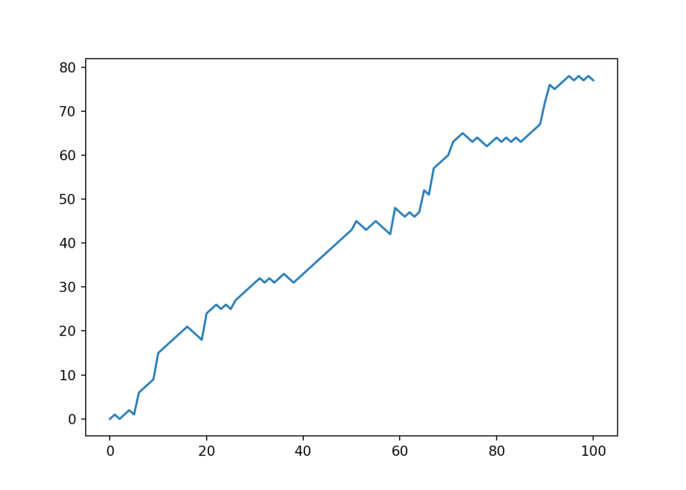
Let’s visualize this random walk! Remember how you could use matplotlib to build a line plot?

import matplotlib.pyplot as plt
plt.plot(x, y)
plt.show()

The first list you pass is mapped onto the x axis and the second list is mapped onto the y axis.

If you pass only one argument, Python will know what to do and will use the index of the list to map onto the x axis, and the values in the list onto the y axis.

# Numpy is imported, seed is set

# Initialization
random_walk = [0]

for x in range(100) :
    step = random_walk[-1]
    dice = np.random.randint(1,7)

    if dice <= 2:
        step = max(0, step - 1)
    elif dice <= 5:
        step = step + 1
    else:
        step = step + np.random.randint(1,7)

    random_walk.append(step)

# Import matplotlib.pyplot as plt

import matplotlib.pyplot as plt

# Plot random_walk

plt.plot(random_walk)

# Show the plot

plt.show()

Simulate multiple walks

A single random walk is one thing, but that doesn’t tell you if you have a good chance at winning the bet.

To get an idea about how big your chances are of reaching 60 steps, you can repeatedly simulate the random walk and collect the results. That’s exactly what you’ll do in this exercise.

The sample code already sets you off in the right direction. Another for loop is wrapped around the code you already wrote. It’s up to you to add some bits and pieces to make sure all of the results are recorded correctly.

Note: Don’t change anything about the initialization of all_walks that is given. Setting any number inside the list will cause the exercise to crash!

# Numpy is imported; seed is set

# Initialize all_walks (don't change this line)
all_walks = []

# Simulate random walk 10 times
for i in range(10) :

    # Code from before
    random_walk = [0]
    for x in range(100) :
        step = random_walk[-1]
        dice = np.random.randint(1,7)

        if dice <= 2:
            step = max(0, step - 1)
        elif dice <= 5:
            step = step + 1
        else:
            step = step + np.random.randint(1,7)
        random_walk.append(step)

    # Append random_walk to all_walks
    all_walks.append(random_walk)

# Print all_walks
print(all_walks)
[[0, 0, 1, 2, 3, 2, 5, 4, 8, 7, 8, 12, 13, 14, 18, 17, 16, 18, 19, 20, 21, 22, 23, 24, 23, 25, 26, 27, 26, 25, 24, 25, 24, 25, 26, 27, 28, 29, 30, 31, 32, 31, 32, 33, 32, 33, 32, 35, 36, 37, 38, 37, 38, 43, 44, 45, 46, 45, 44, 45, 44, 45, 46, 47, 48, 47, 46, 47, 48, 49, 50, 51, 52, 54, 59, 58, 57, 63, 62, 63, 62, 61, 60, 61, 62, 63, 64, 65, 68, 69, 70, 71, 70, 72, 73, 74, 75, 76, 75, 76, 75], [0, 1, 0, 1, 4, 5, 4, 5, 4, 3, 2, 1, 2, 1, 0, 1, 2, 1, 2, 3, 4, 5, 6, 5, 4, 5, 6, 7, 6, 11, 10, 11, 13, 14, 18, 17, 16, 15, 14, 15, 14, 13, 12, 16, 21, 22, 21, 22, 21, 22, 21, 22, 23, 25, 26, 28, 29, 34, 35, 36, 37, 38, 39, 40, 41, 42, 46, 45, 44, 45, 47, 48, 49, 50, 56, 55, 54, 55, 56, 57, 56, 58, 59, 60, 61, 62, 63, 62, 63, 65, 67, 68, 72, 74, 79, 80, 79, 85, 86, 85, 86], [0, 1, 2, 1, 2, 6, 5, 6, 7, 11, 12, 11, 10, 9, 10, 11, 12, 11, 10, 11, 12, 13, 14, 15, 16, 17, 18, 19, 20, 21, 20, 26, 27, 26, 27, 28, 29, 30, 31, 32, 31, 30, 31, 32, 31, 32, 31, 32, 33, 34, 35, 36, 37, 38, 39, 40, 41, 42, 43, 42, 43, 44, 45, 46, 47, 46, 47, 48, 49, 50, 49, 48, 49, 48, 49, 50, 51, 52, 51, 53, 54, 53, 52, 51, 52, 51, 50, 54, 53, 54, 55, 56, 55, 56, 57, 62, 61, 67, 68, 69, 70], [0, 1, 2, 3, 2, 1, 2, 3, 4, 5, 6, 7, 8, 7, 9, 8, 10, 11, 12, 11, 10, 11, 12, 11, 14, 15, 16, 17, 18, 19, 24, 25, 24, 23, 24, 25, 26, 27, 28, 29, 30, 29, 28, 27, 28, 27, 28, 27, 28, 29, 28, 27, 28, 27, 33, 32, 33, 32, 31, 32, 36, 37, 38, 37, 38, 39, 40, 41, 42, 41, 42, 43, 44, 45, 46, 47, 48, 49, 50, 51, 50, 51, 52, 53, 54, 55, 56, 55, 54, 53, 54, 53, 52, 51, 52, 53, 54, 56, 55, 56, 55], [0, 6, 7, 6, 7, 6, 7, 12, 11, 13, 14, 13, 14, 13, 14, 15, 14, 13, 14, 13, 14, 16, 15, 16, 15, 16, 17, 18, 17, 16, 17, 18, 19, 18, 17, 18, 19, 20, 21, 20, 21, 20, 19, 24, 27, 28, 27, 26, 27, 28, 29, 30, 29, 34, 35, 36, 37, 40, 39, 40, 42, 41, 43, 44, 45, 46, 45, 46, 45, 46, 45, 44, 45, 44, 45, 46, 45, 50, 51, 55, 60, 59, 60, 59, 60, 61, 67, 66, 65, 66, 65, 67, 68, 69, 74, 73, 78, 79, 80, 81, 80], [0, 1, 0, 1, 4, 5, 4, 5, 6, 5, 6, 7, 6, 7, 12, 13, 14, 13, 14, 13, 14, 15, 16, 15, 16, 17, 18, 19, 20, 19, 20, 25, 24, 25, 26, 31, 32, 31, 30, 29, 30, 31, 32, 33, 32, 33, 34, 33, 32, 36, 35, 36, 37, 36, 40, 39, 40, 42, 43, 44, 45, 46, 51, 52, 51, 52, 53, 52, 51, 52, 57, 58, 59, 60, 61, 67, 66, 67, 68, 67, 68, 67, 66, 65, 66, 67, 68, 71, 76, 75, 76, 77, 76, 77, 76, 77, 76, 77, 80, 79, 80], [0, 0, 0, 1, 2, 4, 5, 6, 7, 8, 7, 6, 5, 6, 7, 6, 11, 12, 14, 15, 16, 17, 16, 15, 14, 15, 16, 15, 16, 17, 22, 23, 24, 25, 26, 25, 24, 23, 22, 21, 22, 21, 22, 23, 24, 25, 26, 25, 26, 28, 29, 28, 29, 28, 29, 30, 31, 30, 29, 28, 33, 34, 40, 41, 42, 45, 46, 45, 44, 47, 46, 45, 46, 47, 48, 47, 46, 47, 50, 49, 50, 51, 52, 58, 57, 56, 57, 58, 59, 64, 68, 69, 70, 75, 76, 75, 74, 73, 72, 71, 72], [0, 1, 2, 3, 4, 5, 4, 3, 6, 7, 8, 9, 10, 11, 12, 13, 14, 13, 14, 15, 14, 13, 14, 13, 12, 13, 14, 15, 16, 15, 14, 15, 14, 13, 14, 15, 14, 15, 14, 15, 16, 22, 25, 24, 23, 22, 23, 22, 21, 22, 25, 29, 30, 31, 36, 37, 36, 35, 36, 37, 36, 41, 40, 39, 38, 39, 40, 39, 40, 39, 40, 41, 42, 43, 46, 49, 54, 53, 52, 53, 54, 55, 56, 57, 58, 59, 58, 57, 56, 57, 58, 59, 58, 57, 58, 64, 65, 66, 67, 72, 73], [0, 1, 2, 1, 0, 0, 1, 0, 1, 2, 1, 2, 3, 6, 7, 8, 7, 10, 11, 10, 12, 13, 14, 13, 12, 13, 12, 13, 14, 13, 14, 18, 22, 23, 26, 27, 28, 31, 32, 31, 32, 33, 34, 35, 36, 35, 36, 35, 34, 37, 43, 42, 41, 42, 41, 42, 41, 40, 39, 40, 39, 40, 41, 40, 41, 40, 41, 42, 43, 44, 48, 54, 55, 56, 57, 58, 59, 60, 59, 60, 61, 60, 61, 60, 59, 60, 61, 62, 63, 62, 63, 64, 67, 66, 65, 64, 65, 66, 67, 68, 67], [0, 1, 0, 5, 6, 7, 8, 7, 8, 9, 8, 7, 8, 7, 6, 7, 8, 7, 8, 7, 8, 9, 14, 17, 16, 17, 18, 17, 18, 19, 20, 19, 20, 21, 20, 21, 20, 21, 26, 25, 24, 25, 26, 27, 26, 27, 28, 29, 30, 29, 30, 31, 33, 37, 36, 37, 38, 39, 40, 41, 40, 41, 40, 41, 40, 41, 42, 43, 44, 43, 44, 43, 42, 43, 42, 43, 42, 41, 46, 45, 44, 43, 42, 43, 44, 43, 44, 43, 44, 43, 42, 41, 40, 41, 42, 43, 44, 45, 44, 45, 46]]
Visualize all walks

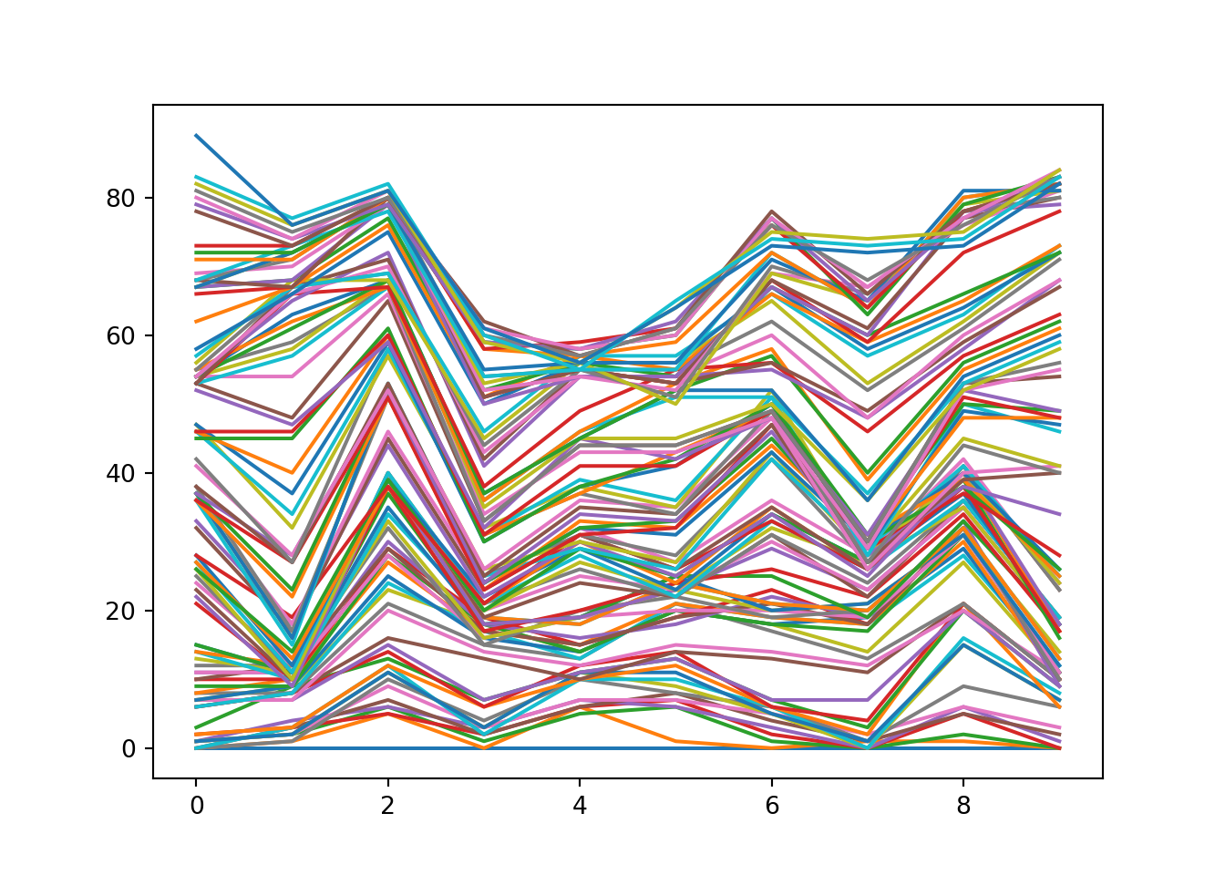
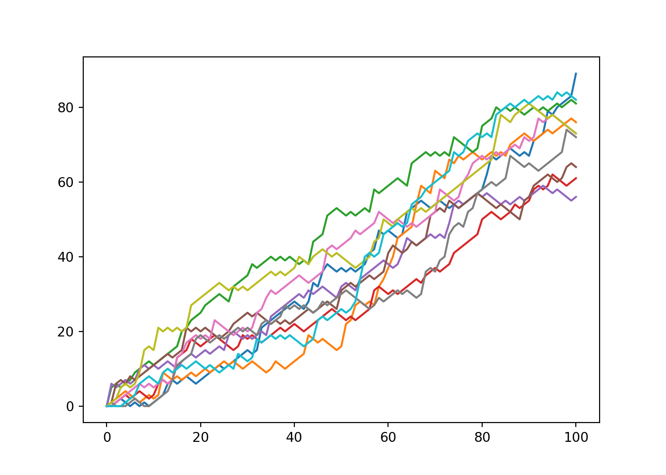
all_walks is a list of lists: every sub-list represents a single random walk. If you convert this list of lists to a NumPy array, you can start making interesting plots! matplotlib.pyplot is already imported as plt.

The nested for loop is already coded for you - don’t worry about it. For now, focus on the code that comes after this for loop.

# numpy and matplotlib imported, seed set.

# initialize and populate all_walks
all_walks = []
for i in range(10) :
    random_walk = [0]
    for x in range(100) :
        step = random_walk[-1]
        dice = np.random.randint(1,7)
        if dice <= 2:
            step = max(0, step - 1)
        elif dice <= 5:
            step = step + 1
        else:
            step = step + np.random.randint(1,7)
        random_walk.append(step)
    all_walks.append(random_walk)

# Convert all_walks to Numpy array: np_aw
np_aw = np.array(all_walks)

# Plot np_aw and show
plt.plot(np_aw)
plt.show()

# Clear the figure
plt.clf()

# Transpose np_aw: np_aw_t

np_aw_t = np.transpose(np_aw)
# Plot np_aw_t and show

plt.plot(np_aw_t)
plt.show()

Implement clumsiness

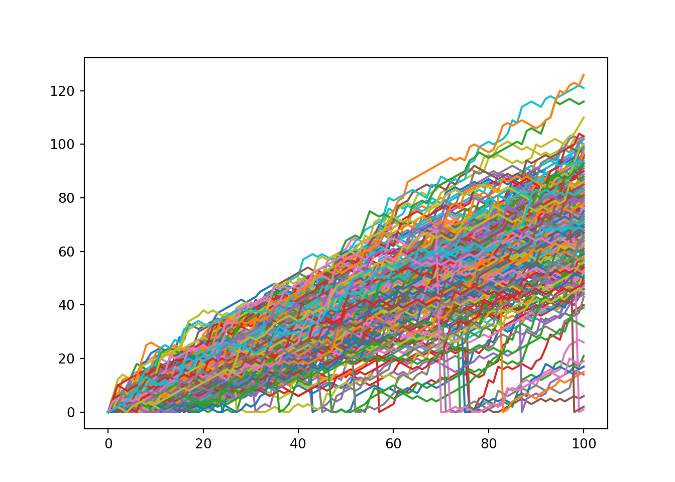
With this neatly written code of yours, changing the number of times the random walk should be simulated is super-easy. You simply update the range() function in the top-level for loop.

There’s still something we forgot! You’re a bit clumsy and you have a 0.5% chance of falling down. That calls for another random number generation. Basically, you can generate a random float between 0 and 1. If this value is less than or equal to 0.005, you should reset step to 0.

# numpy and matplotlib imported, seed set

# Simulate random walk 250 times
all_walks = []
for i in range(250) :
    random_walk = [0]
    for x in range(100) :
        step = random_walk[-1]
        dice = np.random.randint(1,7)
        if dice <= 2:
            step = max(0, step - 1)
        elif dice <= 5:
            step = step + 1
        else:
            step = step + np.random.randint(1,7)

        # Implement clumsiness
        if np.random.rand() <= 0.001 :
            step = 0

        random_walk.append(step)
    all_walks.append(random_walk)

# Create and plot np_aw_t
np_aw_t = np.transpose(np.array(all_walks))
plt.plot(np_aw_t)
plt.show()

Plot the distribution

All these fancy visualizations have put us on a sidetrack. We still have to solve the million-dollar problem: What are the odds that you’ll reach 60 steps high on the Empire State Building?

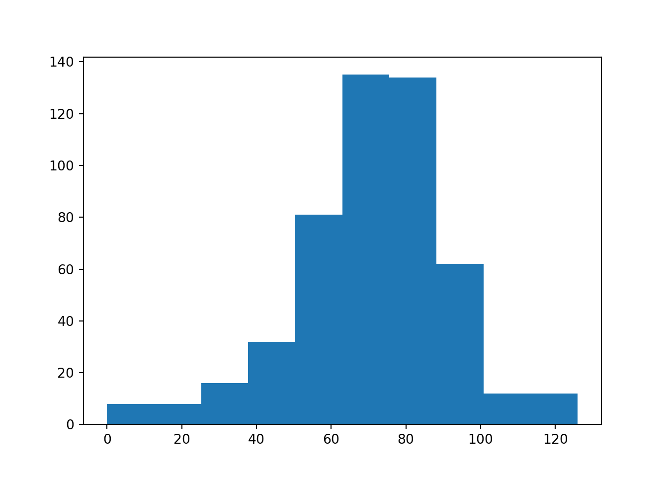
Basically, you want to know about the end points of all the random walks you’ve simulated. These end points have a certain distribution that you can visualize with a histogram.

Note that if your code is taking too long to run, you might be plotting a histogram of the wrong data!

# numpy and matplotlib imported, seed set

# Simulate random walk 500 times
all_walks = []
for i in range(500) :
    random_walk = [0]
    for x in range(100) :
        step = random_walk[-1]
        dice = np.random.randint(1,7)
        if dice <= 2:
            step = max(0, step - 1)
        elif dice <= 5:
            step = step + 1
        else:
            step = step + np.random.randint(1,7)
        if np.random.rand() <= 0.001 :
            step = 0
        random_walk.append(step)
    all_walks.append(random_walk)

# Create and plot np_aw_t
np_aw_t = np.transpose(np.array(all_walks))

# Select last row from np_aw_t: ends
ends = np_aw_t[100,:]

# Plot histogram of ends, display plot
plt.hist(ends)
plt.show()

Calculate the odds

The histogram of the previous exercise was created from a NumPy array ends, that contains 500 integers. Each integer represents the end point of a random walk. To calculate the chance that this end point is greater than or equal to 60, you can count the number of integers in ends that are greater than or equal to 60 and divide that number by 500, the total number of simulations.

Well then, what’s the estimated chance that you’ll reach at least 60 steps high if you play this Empire State Building game? The ends array is everything you need; it’s available in your Python session so you can make calculations in the IPython Shell.

round(len(ends[ends>=60])/len(ends) * 100, 2)
75.8