Writing Efficient R Code

Author

Mburu

Published

August 13, 2021

R version

One of the relatively easy optimizations available is to use an up-to-date version of R. In general, R is very conservative, so upgrading doesn’t break existing code. However, a new version will often provide free speed boosts for key functions.

The version command returns a list that contains (among other things) the major and minor version of R currently being used.

# Print the R version details using version
version

               _                           
platform       x86_64-pc-linux-gnu         
arch           x86_64                      
os             linux-gnu                   
system         x86_64, linux-gnu           
status                                     
major          4                           
minor          3.0                         
year           2023                        
month          04                          
day            21                          
svn rev        84292                       
language       R                           
version.string R version 4.3.0 (2023-04-21)
nickname       Already Tomorrow

# Assign the variable major to the major component
major <- version$major

# Assign the variable minor to the minor component
minor <- version$minor

Comparing read times of CSV and RDS files

One of the most common tasks we perform is reading in data from CSV files. However, for large CSV files this can be slow. One neat trick is to read in the data and save as an R binary file (rds) using saveRDS(). To read in the rds file, we use readRDS().

Note: Since rds is R’s native format for storing single objects, you have not introduced any third-party dependencies that may change in the future.

To benchmark the two approaches, you can use system.time(). This function returns the time taken to evaluate any R expression. For example, to time how long it takes to calculate the square root of the numbers from one to ten million, you would write the following:

# How long does it take to read movies from CSV?
system.time(read.csv("movies.csv"))

   user  system elapsed 
  0.152   0.008   0.160

# How long does it take to read movies from RDS?
system.time(readRDS("movies.rds"))

   user  system elapsed 
  0.037   0.000   0.036

Elapsed time

Using system.time() is convenient, but it does have its drawbacks when comparing multiple function calls. The microbenchmark package solves this problem with the microbenchmark() function.

# Load the microbenchmark package
library(microbenchmark)

# Compare the two functions
compare <- microbenchmark(read.csv("movies.csv"), 
                          readRDS("movies.rds"), 
                          times = 100)

# Print compare
compare

Unit: milliseconds
                   expr       min        lq      mean    median        uq
 read.csv("movies.csv") 148.89375 157.21866 175.08927 164.73617 183.27556
  readRDS("movies.rds")  35.01906  36.63868  39.98763  38.80657  40.00251
       max neval
 371.18248   100
  82.90037   100

My hardware For many problems your time is the expensive part. If having a faster computer makes you more productive, it can be cost effective to buy one. However, before you splash out on new toys for yourself, your boss/partner may want to see some numbers to justify the expense. Measuring the performance of your computer is called benchmarking, and you can do that with the benchmarkme package.

# Load the benchmarkme package
library(benchmarkme)

# Assign the variable ram to the amount of RAM on this machine
ram <- get_ram()
ram

16.5 GB

# Assign the variable cpu to the cpu specs
cpu <- get_cpu()
cpu

$vendor_id
[1] "GenuineIntel"

$model_name
[1] "11th Gen Intel(R) Core(TM) i7-11370H @ 3.30GHz"

$no_of_cores
[1] 8

Benchmark DataCamp’s machine

The benchmarkme package allows you to run a set of standardized benchmarks and compare your results to other users. One set of benchmarks tests is reading and writing speeds.

The function call

res = benchmark_io(runs = 1, size = 5) records the length of time it takes to read and write a 5MB file.

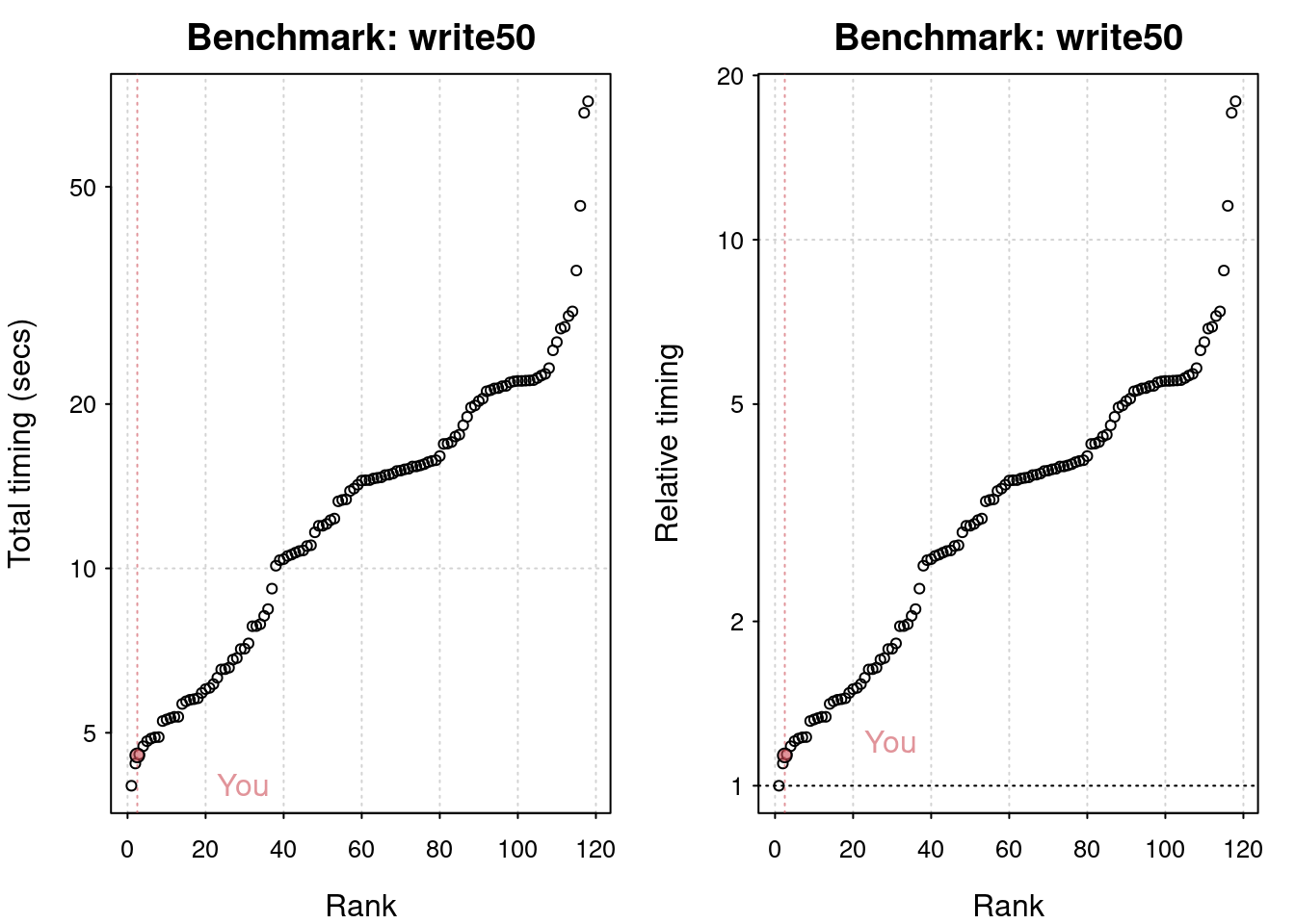
# Run the io benchmark
res <- benchmark_io(runs = 1, size = 50)

Preparing read/write io

# IO benchmarks (2 tests) for size 50 MB:

     Writing a csv with 6250000 values: 4.55 (sec).

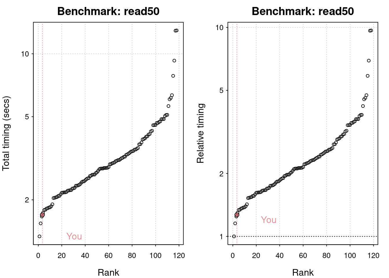
     Reading a csv with 6250000 values: 1.7 (sec).

# Plot the results
plot(res)

You are ranked 3 out of 119 machines.

Press return to get next plot

You are ranked 4 out of 119 machines.

Benchmark r operations

# Run each benchmark 3 times
res <- benchmark_std(runs = 10)

# Programming benchmarks (5 tests):

    3,500,000 Fibonacci numbers calculation (vector calc): 0.154 (sec).

    Grand common divisors of 1,000,000 pairs (recursion): 0.467 (sec).

    Creation of a 3,500 x 3,500 Hilbert matrix (matrix calc): 0.194 (sec).

    Creation of a 3,000 x 3,000 Toeplitz matrix (loops): 0.976 (sec).

    Escoufier's method on a 60 x 60 matrix (mixed): 0.869 (sec).

# Matrix calculation benchmarks (5 tests):

    Creation, transp., deformation of a 5,000 x 5,000 matrix: 0.282 (sec).

    2,500 x 2,500 normal distributed random matrix^1,000: 0.16 (sec).

    Sorting of 7,000,000 random values: 0.556 (sec).

    2,500 x 2,500 cross-product matrix (b = a' * a): 8.03 (sec).

    Linear regr. over a 5,000 x 500 matrix (c = a \ b'): 0.695 (sec).

# Matrix function benchmarks (5 tests):

    Cholesky decomposition of a 3,000 x 3,000 matrix: 4.43 (sec).

    Determinant of a 2,500 x 2,500 random matrix: 2.64 (sec).

    Eigenvalues of a 640 x 640 random matrix: 0.515 (sec).

    FFT over 2,500,000 random values: 0.168 (sec).

    Inverse of a 1,600 x 1,600 random matrix: 2.39 (sec).

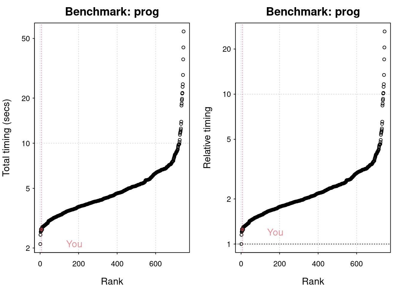
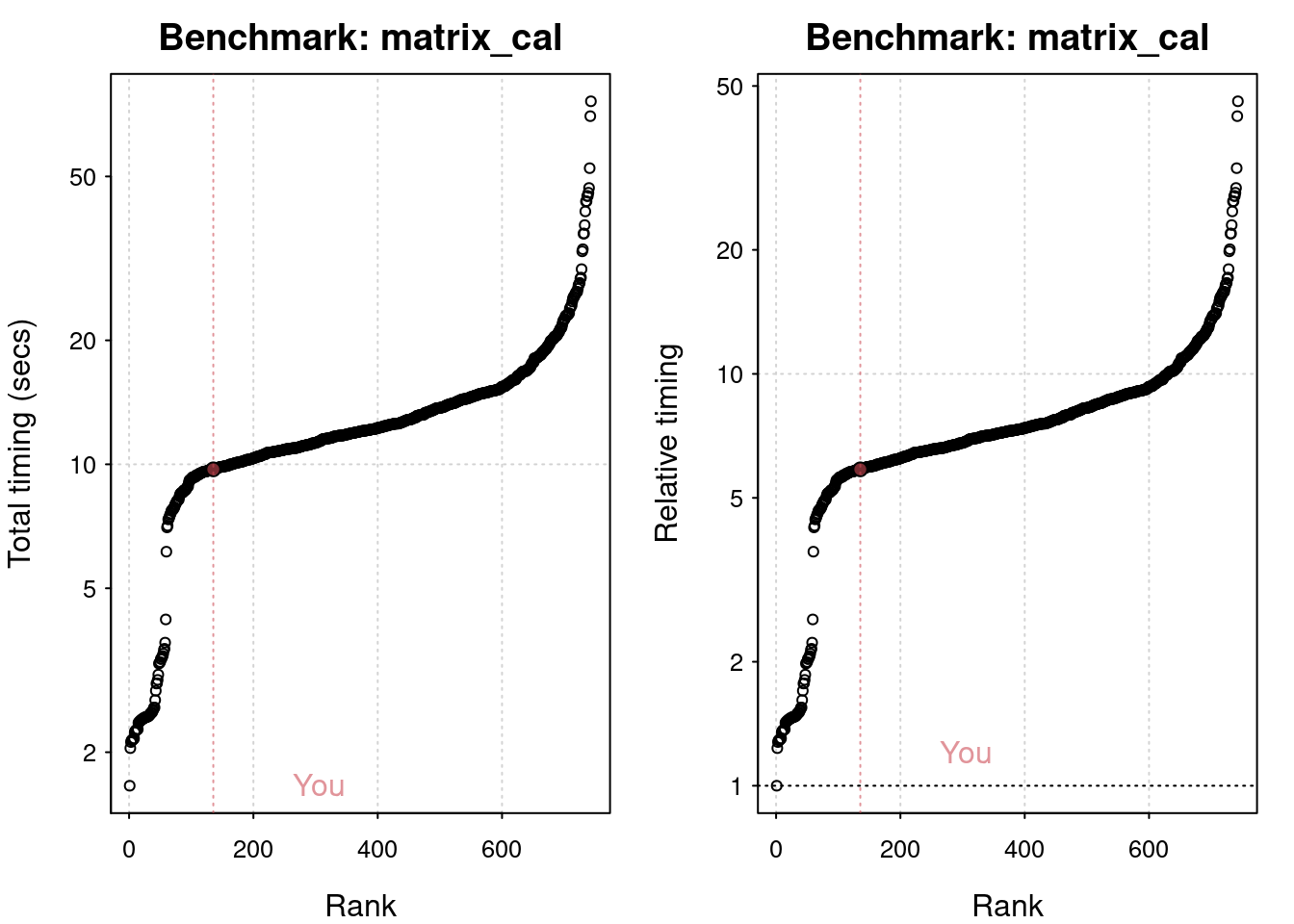
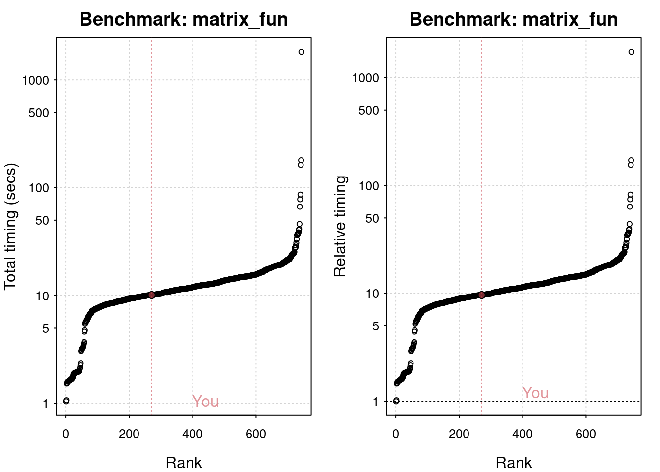
plot(res)

You are ranked 8 out of 749 machines.

Press return to get next plot

You are ranked 136 out of 747 machines.

Press return to get next plot

You are ranked 271 out of 747 machines.

Timings - growing a vector

Growing a vector is one of the deadly sins in R; you should always avoid it.

The growing() function defined below generates n random standard normal numbers, but grows the size of the vector each time an element is added!

Note: Standard normal numbers are numbers drawn from a normal distribution with mean 0 and standard deviation 1.

n <- 30000 # Slow code growing <- function(n) { x <- NULL for(i in 1:n) x <- c(x, rnorm(1)) x }

growing <- function(n) {
    x = NULL
    for(i in 1:n) 
        x = c(x, rnorm(1))
    x
}

# Use <- with system.time() to store the result as res_grow
system.time(res_grow <- growing(30000))

   user  system elapsed 
  0.776   0.000   0.776

Timings - pre-allocation In the previous exercise, growing the vector took around 2 seconds. How long does it take when we pre-allocate the vector? The pre_allocate() function is defined below.

n <- 30000
# Fast code
pre_allocate <- function(n) {
    x <- numeric(n) # Pre-allocate
    for(i in 1:n) 
        x[i] <- rnorm(1)
    x
}


# Use <- with system.time() to store the result as res_allocate
n <- 30000
system.time(res_allocate <- pre_allocate(n))

   user  system elapsed 
   0.04    0.00    0.04

Vectorized code: multiplication

The following piece of code is written like traditional C or Fortran code. Instead of using the vectorized version of multiplication, it uses a for loop.

Your job is to make this code more “R-like” by vectorizing it.

x <- rnorm(10)
x2 <- numeric(length(x))
for(i in 1:10)
    x2[i] <- x[i] * x[i]
# Store your answer as x2_imp
x2_imp <- x*x

Vectorized code: calculating a log-sum

A common operation in statistics is to calculate the sum of log probabilities. The following code calculates the log-sum (the sum of the logs).

x is a vector of probabilities

total <- 0 for(i in seq_along(x)) total <- total + log(x\[i\]) However this piece of code could be significantly improved using vectorized code.

# Initial code
n <- 100
total <- 0
x <- runif(n)
for(i in 1:n) 
    total <- total + log(x[i])

# Rewrite in a single line. Store the result in log_sum
log_sum <- sum(log(x))

Data frames and matrices - column selection

All values in a matrix must have the same data type, which has efficiency implications when selecting rows and columns.

Suppose we have two objects, mat (a matrix) and df (a data frame).

# Which is faster, mat[, 1] or df[, 1]? 
microbenchmark(mat[, 1], df[, 1])

Row timings

Similar to the previous example, the objects mat and df are a matrix and a data frame, respectively. Using microbenchmark(), how long does it take to select the first row from each of these objects?

To make the comparison fair, just use mat\[1, \] and df\[1, \].

Interesting! Accessing a row of a data frame is much slower than accessing that of a matrix, more so than when accessing a column from each data type. This is because the values of a column of a data frame must be the same data type, whereas that of a row doesn’t have to be. Do you see the pattern here?

# Which is faster, mat[, 1] or df[, 1]? 
microbenchmark(mat[1, ], df[1, ])

Profvis in action

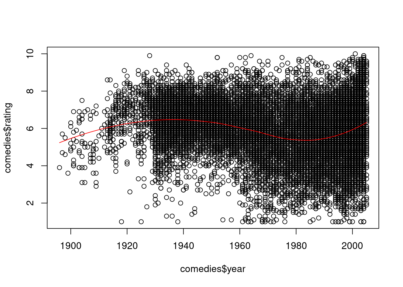
Examine the code on the right that performs a standard data analysis. It loads and selects data, plots the data of interest, and adds in a regression line.

# Load the data set
data(movies, package = "ggplot2movies") 

# Load the profvis package
library(profvis)

# Profile the following code with the profvis function
profvis({
  # Load and select data
  comedies <- movies[movies$Comedy == 1, ]

  # Plot data of interest
  plot(comedies$year, comedies$rating)

  # Loess regression line
  model <- loess(rating ~ year, data = comedies)
  j <- order(comedies$year)
  
  # Add fitted line to the plot
  lines(comedies$year[j], model$fitted[j], col = "red")
})    ## Remember the closing brackets!